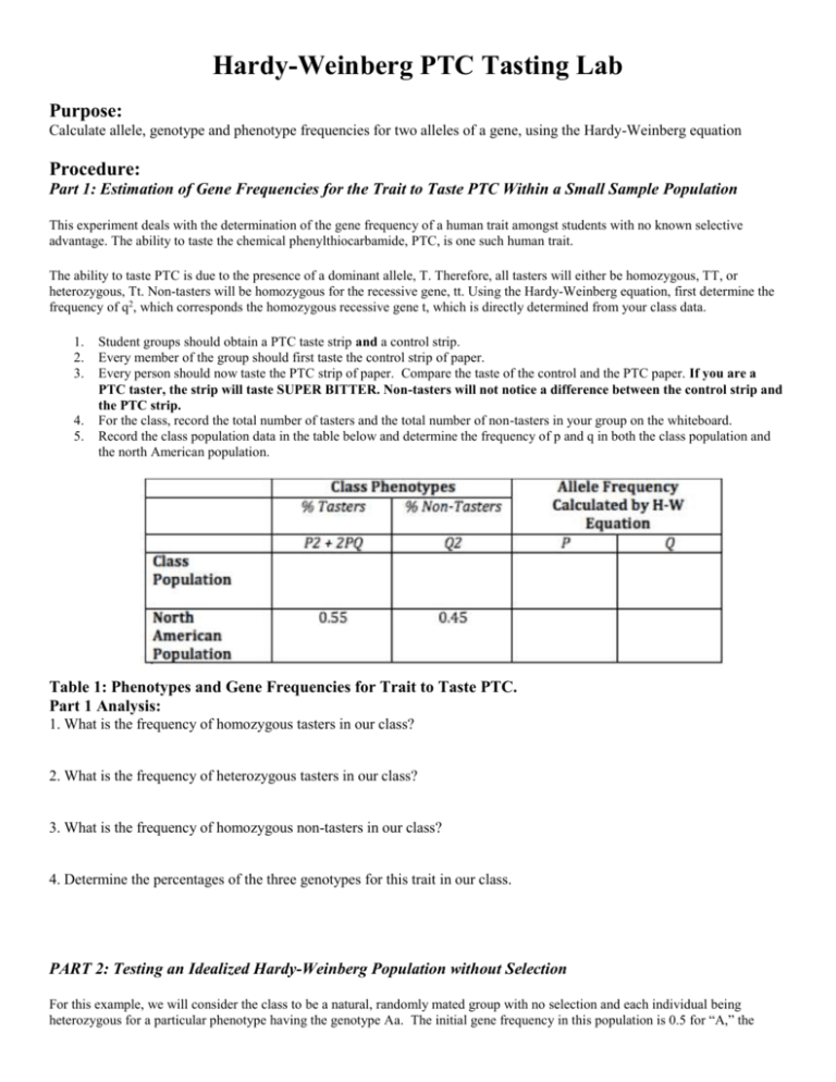
Hardy-Weinberg PTC Tasting Lab
Purpose:
Calculate allele, genotype and phenotype frequencies for two alleles of a gene, using the Hardy-Weinberg equation
Procedure:
Part 1: Estimation of Gene Frequencies for the Trait to Taste PTC Within a Small Sample Population
This experiment deals with the determination of the gene frequency of a human trait amongst students with no known selective
advantage. The ability to taste the chemical phenylthiocarbamide, PTC, is one such human trait.
The ability to taste PTC is due to the presence of a dominant allele, T. Therefore, all tasters will either be homozygous, TT, or
heterozygous, Tt. Non-tasters will be homozygous for the recessive gene, tt. Using the Hardy-Weinberg equation, first determine the
frequency of q2, which corresponds the homozygous recessive gene t, which is directly determined from your class data.
1.
2.
3.
4.
5.
Student groups should obtain a PTC taste strip and a control strip.
Every member of the group should first taste the control strip of paper.
Every person should now taste the PTC strip of paper. Compare the taste of the control and the PTC paper. If you are a
PTC taster, the strip will taste SUPER BITTER. Non-tasters will not notice a difference between the control strip and
the PTC strip.
For the class, record the total number of tasters and the total number of non-tasters in your group on the whiteboard.
Record the class population data in the table below and determine the frequency of p and q in both the class population and
the north American population.
Table 1: Phenotypes and Gene Frequencies for Trait to Taste PTC.
Part 1 Analysis:
1. What is the frequency of homozygous tasters in our class?
2. What is the frequency of heterozygous tasters in our class?
3. What is the frequency of homozygous non-tasters in our class?
4. Determine the percentages of the three genotypes for this trait in our class.
PART 2: Testing an Idealized Hardy-Weinberg Population without Selection
For this example, we will consider the class to be a natural, randomly mated group with no selection and each individual being
heterozygous for a particular phenotype having the genotype Aa. The initial gene frequency in this population is 0.5 for “A,” the
dominant allele and 0.5 for “a,” the recessive allele. Therefore p and q both equal 0.5. Every pair of individuals should keep track of
their child’s genotype after each mating. In addition, the class as a group must keep track of totals for each mating during each of the
five generations.
1.
2.
3.
4.
5.
6.
7.
8.
9.
10.
11.
12.
13.
14.
Work in pairs. For each generation, each pair will produce two offspring.
For this example, each person in the class should obtain 4 index cards. Label two “A” and two “a.” These cards represent
the only two unique gametes with a heterozygous individual with a genotype of Aa can produce.
Each person in a group of two should place the index cards face down on a flat surface. Shuffle cards so that they are
randomly mixed. Each person selects only one card from their pile of 4 cards and places it together with the one
selected by your partner.
Flip the cards over and record the genotype of this mating in Table 2.
Recover your index card so again you have two of each allele “A”, and “a.” Reshuffle the cards between selections.
With your partner, produce a second offspring and record the genotype. Be sure to collect the class totals on the whiteboard at
the end of this generation and for the next 4 generations.
Now you will assume the genotype of the first child and your partner will assume the genotype of the second child.
Re-label your four index cards to reflect the gametes which you would produce with the new genotype. For example if your
child was AA, your cards would be labeled A,A,A,A. Similarly, if your child was Aa, your cards would be labeled A,A,a,a.
Now, things are going to get a little weird. Randomly find someone else in class to mate with. If someone approaches you
with a twinkle in their eye and says, “How’s about you and me?” Your reply should be, “Absolutely.” We have to be a little
promiscuous in this simulation to model real population dynamics. Random mating is key.
Using the same procedure for the first generation, produce two new offspring with your new mate. Again record the
genotype of each child in the table. Remember, the class as a group should also keep track of each genotype after each
generation. Record the class totals.
As before, one student of the pair will assume the genotype of the first child and the other student should assume the
genotype of the second child produced during the mating. If necessary, re-label your index cards to reflect the four gametes
which you would produce.
Again, each person should randomly seek out another mate and repeat the procedure generating two new children. Record the
new genotypes as before. Keep track of the class totals after each mating.
This process of “random mating” without selection should continue until you have produced 5 generations of children.
Be sure to place your individual results and the class totals for each mating into Table 2.
Analysis
1.
Calculate, from your experimental data, gene frequency values of the “A” and “a” alleles, as well as p and q in your class
population. These can be obtained by using the following formulas to determine A (p) and a (q) frequencies:
a)
A Frequency = (Total number of AA individuals x 2) + (Total number of Aa individuals) / (Total number of all individuals)
b) a Frequency = (Total number of aa individuals x 2) + (Total number of Aa individuals) / (Total number of all individuals)
2.
Determine the theoretical Hardy-Weinberg frequencies of the “Class Totals for each Genotype added over 5 Generations”:
1.
2.
3.
p2 (AA): __________________
2pq (AA): _________________
q2 (aa): ___________________
3.
Determine p and q for “Class Totals for each Genotype added over 5 Generations”:
1.
2.
p: ___________________
q: ___________________
4. Determine the theoretical Hardy-Weinberg frequencies of the beginning population when p=0.5, and q=0.5.
1.
2.
3.
p2 (AA): ___________________
2pq (Aa): __________________
q2 (aa): ____________________
5.
Calculate the genotype frequencies in Part 2 from the 5th generation only:
1.
2.
3.
AA: ___________________
Aa: ___________________
aa: ___________________
6.
How do the values from all of the generations added together compare to 5th generation? Have they changed? How?
We’ll continue with parts 3 and 4 on Monday.
Part 3: Testing an Idealized Hardy-Weinberg Population with Selection
Now that you have the facts of life well in hand, we can begin to modify our simulation, making it more
realistic and enable us to investigate some basic questions about selection and gene frequencies. In humans,
there are several genetic “diseases” that have been thoroughly investigated. One good example is sickle-cell
anemia. This is a single allele trait; the homozygous recessive genotype is lethal, and the afflicted individual
usually dies prior to reaching reproductive maturity. Both the homozygous dominant and the heterozygote
survive. At this point, we will consider both the homozygous dominant and the heterozygote phenotypically
identical. In other words, we are selecting against the homozygote recessive 100% of the time.
The procedure is similar to Part 2. Start again with your initial genotype, and choose the genotype of your
offspring as in Part 2. This time, however, there is one important difference. Every time your offspring is aa it
dies. Since we want to maintain a constant population size, the same two parents must try again until they
produce a surviving offspring.
As you might already have realized, there is one real problem that must be solved before we begin. 25% of you
are already homozygous recessive or dead! There are two ways we could deal with this:
(a) We could reassign genotypes so that no one starts with aa, but then our original population would not follow
a Hardy-Weinberg distribution, prohibiting any comparisons between Part 2 and Part 3.
(b) Instead, we will make the assumption that aa in the initial parent is not lethal, and that two aa individuals
cannot mate. In other words, if you are aa, just be sure not to mate with another aa in the first round.
Proceed through five generations, selecting against the homozygous recessive offspring. Now, add up the
genotype frequencies that exist in the population and calculate the new p and q.
Analysis
1. How do the new p and q compare to the values in Case I?
2. Has the population changed?
3. What would happen to the p and q if we went another five generations?
4. In a large population, what are the chances of eliminating completely a deleterious recessive allele?
Part 4: Testing an Idealized Hardy-Weinberg Population with a Heterozygous Advantage
From Part 3, it is easy to see that the lethal recessive allele rapidly decreases in the population. However, data
from many human populations show an unexpectedly high frequency of the sickle-cell allele present in some
populations. In other words, our simulation does not accurately reflect the real situation. The heterozygote is
slightly more resistant to a deadly form of malaria than the homozygous dominant individual. In other words,
there is a slight selection against the homozygous dominant individual as compared to the heterozygote. This
fact is easily incorporated into our simulation. In this round, keep everything the same as in Part 3, except that
if your offspring is AA, flip a coin. Heads he lives, tails he dies of malaria, and the same parents must mate
again until they get a viable offspring.
Go through five generations, starting again with your initial genotype. The genotype aa dies 100% of the time.
After five generations, total the genotypes and calculate p and q. Now, starting with the genotype you last had,
go through five more generations, and again total the genotypes and calculate p and q. If time permits, another
five generations is extremely informative.
Analysis
1. How do p and q in Part 3 compare with Part 2 and Part 4?
2. Do you think the recessive allele will be completely eliminated in either Part 3 or Part 4?
3. What is the importance of heterozygous advantage in maintaining genetic variation in populations?
Part 5 (Time permitting) – Genetic Drift
In Part 2, the role of small populations in genetic drift was suggested. It is possible to use our simulation to
look at this phenomenon in more detail. Divide the lab into several smaller populations (For example, a class of
30 could be divided into 3 populations of 10 each.) When the populations are reproductively isolated by
mountain ranges, oceans, or imaginary walls, total the genotypic and allelic frequencies in each population.
Now go through five generations as in Part 2. Record the new genotypic frequencies, and calculate the new p
and q for each population.
Analysis
1. How did the initial genotypic frequencies of the populations compare?
2. What do your results indicate about the importance of populations size as an evolutionary force?