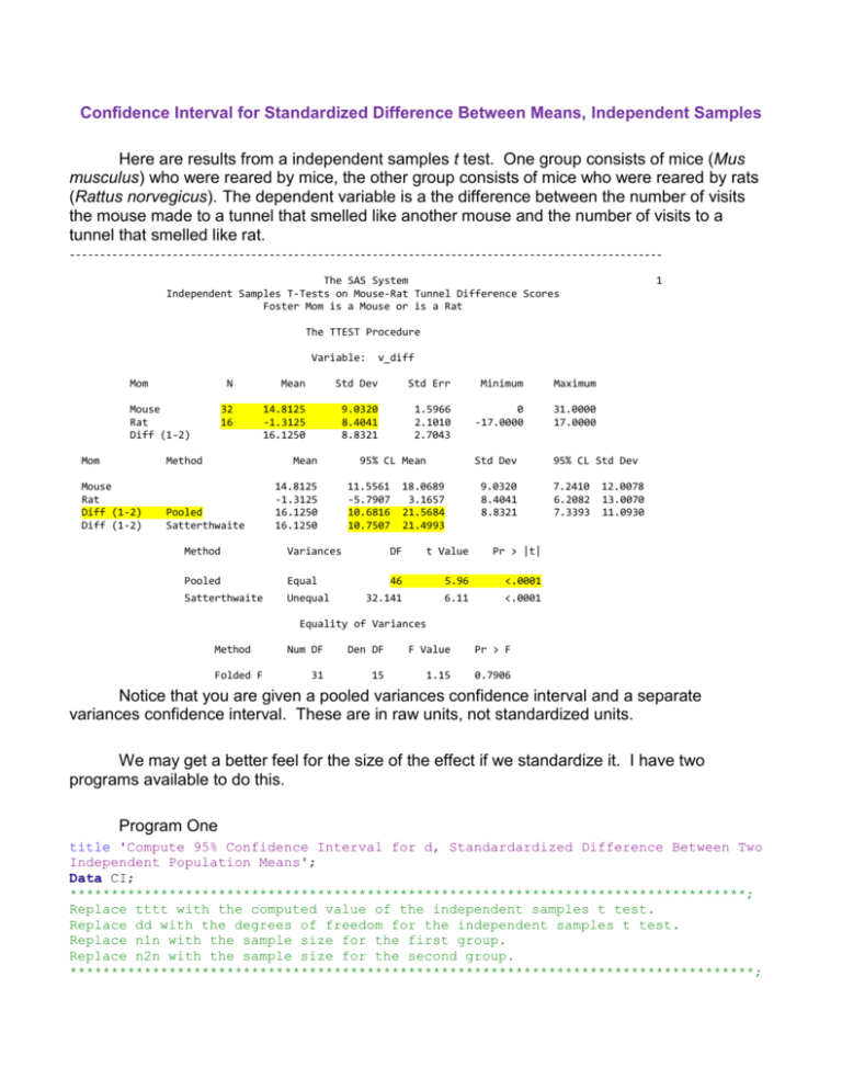
Confidence Interval for Standardized Difference Between Means, Independent Samples
Here are results from a independent samples t test. One group consists of mice (Mus
musculus) who were reared by mice, the other group consists of mice who were reared by rats
(Rattus norvegicus). The dependent variable is a the difference between the number of visits
the mouse made to a tunnel that smelled like another mouse and the number of visits to a
tunnel that smelled like rat.
-------------------------------------------------------------------------------------------------The SAS System
Independent Samples T-Tests on Mouse-Rat Tunnel Difference Scores
Foster Mom is a Mouse or is a Rat
1
The TTEST Procedure
Variable:
Mom
Mouse
Rat
Diff (1-2)
Mom
N
Mean
Std Dev
Std Err
Minimum
Maximum
32
16
14.8125
-1.3125
16.1250
9.0320
8.4041
8.8321
1.5966
2.1010
2.7043
0
-17.0000
31.0000
17.0000
Std Dev
95% CL Std Dev
Method
Mouse
Rat
Diff (1-2)
Diff (1-2)
v_diff
Mean
Pooled
Satterthwaite
14.8125
-1.3125
16.1250
16.1250
Method
Variances
Pooled
Equal
Satterthwaite
Unequal
95% CL Mean
11.5561
-5.7907
10.6816
10.7507
18.0689
3.1657
21.5684
21.4993
DF
9.0320
8.4041
8.8321
t Value
7.2410
6.2082
7.3393
12.0078
13.0070
11.0930
Pr > |t|
46
5.96
<.0001
32.141
6.11
<.0001
Equality of Variances
Method
Folded F
Num DF
Den DF
F Value
Pr > F
31
15
1.15
0.7906
Notice that you are given a pooled variances confidence interval and a separate
variances confidence interval. These are in raw units, not standardized units.
We may get a better feel for the size of the effect if we standardize it. I have two
programs available to do this.
Program One
title 'Compute 95% Confidence Interval for d, Standardardized Difference Between Two
Independent Population Means';
Data CI;
**********************************************************************************;
Replace tttt with the computed value of the independent samples t test.
Replace dd with the degrees of freedom for the independent samples t test.
Replace n1n with the sample size for the first group.
Replace n2n with the sample size for the second group.
***********************************************************************************;
t= 5.96 ;
df = 46 ;
n1 = 32 ;
n2 = 16 ;
***********************************************************************************;
g = t/sqrt(n1*n2/(n1+n2));
ncp_lower = TNONCT(t,df,.975);
ncp_upper = TNONCT(t,df,.025);
d_lower = ncp_lower*sqrt((n1+n2)/(n1*n2));
d_upper = ncp_upper*sqrt((n1+n2)/(n1*n2));
output; run; proc print; var g d_lower d_upper; run;
The Output
Obs
g
d_lower
d_upper
1
1.82487
1.11164
2.52360
Notice that both sides of the confidence interval indicate that the effect is quite large.
Program 2
*This program computes a CI for the effect size in
a between-subject design with two groups.
m1 and m2 are the means for the two groups
s1 and s2 are the standard deviations for the two groups
n1 and n2 are the sample sizes for the two groups
prob is the confidence level;
*Downloaded from James Algina’s webpage at http://plaza.ufl.edu/algina/ ;
data;
m1=14.8125
;
m2= -1.3125
;
s1=9.032
;
s2=8.4041
;
n1=32 ;
n2=16 ;
prob=.95;
v1=s1**2;
v2=s2**2;
pvar=((n1-1)*v1+(n2-1)*v2)/(n1+n2-2);
se=sqrt(pvar*(1/n1+1/n2));
nchat=(m1-m2)/se;
es=(m1-m2)/(sqrt(pvar));
df=n1+n2-2;
ncu=TNONCT(nchat,df,(1-prob)/2);
ncl=TNONCT(nchat,df,1-(1-prob)/2);
ll=(sqrt(1/n1+1/n2))*ncl;
ul=(sqrt(1/n1+1/n2))*ncu;
output;
proc print;
title1 'll is the lower limit and ul is the upper limit';
title2 'of a confidence interval for the effect size';
var es ll ul;
run;
The Output
ll is the lower limit and ul is the upper limit
of a confidence interval for the effect size
Obs
es
ll
ul
1
1.82572
1.11239
2.52453
2
The minor differences between these results and those shown earlier are due to rounding error
from the value of t.


Do it with SPSS
Wuensch’s Stats Lessons
Karl L. Wuensch, East Carolina University, Dept. of Psychology, 3. September, 2011.