Standardized Effect Size Estimates for Repeated Measures ANOVA
Grissom and Kim (2012) discuss effect sizes for repeated measures ANOVA in their book Effect Sizes
for Research (pages 196 through 201). The only effect size estimate for which they indicate how to construct
confidence intervals is that developed by Algina and Kesleman (2003), which constructs confidence intervals
for multiple contrasts between groups. The estimated effect size parameter is the standardized difference
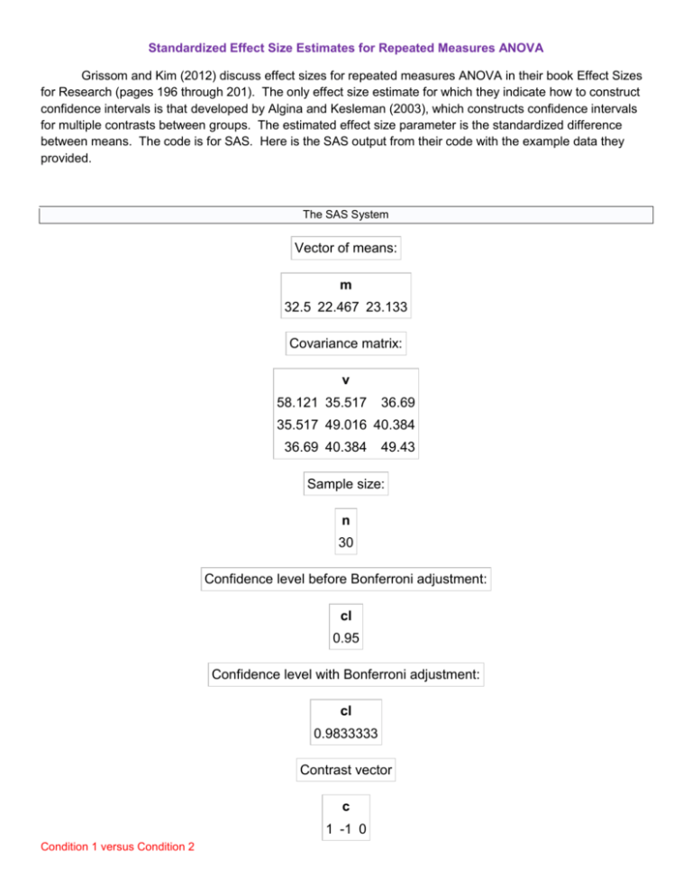
between means. The code is for SAS. Here is the SAS output from their code with the example data they
provided.
The SAS System
Vector of means:
m
32.5 22.467 23.133
Covariance matrix:
v
58.121 35.517
36.69
35.517 49.016 40.384
36.69 40.384
49.43
Sample size:
n
30
Confidence level before Bonferroni adjustment:
cl
0.95
Confidence level with Bonferroni adjustment:
cl
0.9833333
Contrast vector
c
1 -1 0
Condition 1 versus Condition 2
Effect size:
es
1.3888052
Estimated noncentrality parameter
nchat
9.1457599
ll is the lower limit of the CI and ul is the upper limit
ll
ul
0.8219189 1.9544733
Contrast vector
c
1 0 -1
Condition 1 versus Condition 3
Effect size:
es
1.296615
Estimated noncentrality parameter
nchat
8.7767212
ll is the lower limit of the CI and ul is the upper limit
ll
ul
0.7577019 1.8336671
Contrast vector
c
0 1 -1
Condition 2 versus Condition 3
Effect size:
es
-0.09219
Estimated noncentrality parameter
nchat
-0.867597
ll is the lower limit of the CI and ul is the upper limit
ll
ul
-0.347428 0.1645981
The Code
* This program is used with within-subjects designs. It computes
confidence intervals for effect size estimates. To use the program one
inputs at the top of the program:
m--a vector of means
v--a covariance matrix in lower diagonal form, with periods for
the upper elements
n--the sample size
prob--the confidence level prior to the Bonferroni adjustment
adjust--the number of contrats is a Bonferroni adjustment to the
confidence level is requested. Otherwise adjust is set
equal to 1
Bird--a switch that uses the variances of all variables to calculate
the denominator of the effect size as suggested by K. Bird
(Bird=1). Our suggestion is to use the variance of those
variables involved in the contrast to calculate the denominator
of the effect size (Bird=0)
In addition one inputs at the bottom of the program:
c--a vector of contrast weights
multiple contrasts can be entered. After each, type the code
run ci;
*Downloaded from James Algina's page at http://plaza.ufl.edu/algina/index.programs.html ;
*************************************************************************************;
proc iml;
m={32.500 22.467 23.133};
v={58.121 . .,
35.517 49.016 .,
36.690 40.384 49.430};
do ii = 1 to nrow(v)-1;
do jj = ii+1 to nrow(v);
v[ii,jj]=v[jj,ii];
end;
end;
n=30 ;
Bird=1;
df=n-1;
cl=.95;
adjust=3;
prob=cl;
print 'Vector of means:';
print m;
print 'Covariance matrix:';
print v;
print 'Sample size:';
print n;
print 'Confidence level before Bonferroni adjustment:';
print cl;
cl=1-(1-prob)/adjust;
print 'Confidence level with Bonferroni adjustment:';
print cl;
start CI;
pvar=0;
count=0;
if bird=0 then do;
do mm=1 to nrow(v);
if c[1,mm]^=0 then do;
pvar=pvar+v[mm,mm];
count=count+1;
end;
end;
end;
if bird=1 then do;
do mm=1 to nrow(v);
pvar=pvar+v[mm,mm];
count=count+1;
end;
end;
pvar=pvar/count;
es=m*c`/(sqrt(pvar));
se=sqrt(c*v*c`/n);
nchat=m*c`/se;
ncu=TNONCT(nchat,df,(1-prob)/(2*adjust));
ncl=TNONCT(nchat,df,1-(1-prob)/(2*adjust));
ll=se*ncl/(sqrt(pvar));
ul=se*ncu/(sqrt(pvar));
print 'Contrast vector';
print c;
print 'Effect size:';
print es;
Print 'Estimated noncentrality parameter';
print nchat;
Print 'll is the lower limit of the CI and ul is the upper limit';
print ll ul;
finish;
c={1 -1 0};
run ci;
c={1 0 -1};
run ci;
c={0 1 -1};
run ci;
quit;
References
Algina, J., & Keselman, H. J. (2003). Approximate confidence intervals for effect sizes. Educational
and Psychological Measurement, 63, 537-553. DOI: 10.1177/0013164403256358
Grissom, R. J., & Kim, J. J. (2012). Effect sizes for research: Univariate and multivariate applications
(2nd ed.). New York, NY: Routledge.
Karl L. Wuensch, November, 2015
Wuensch’s Stat Lessons