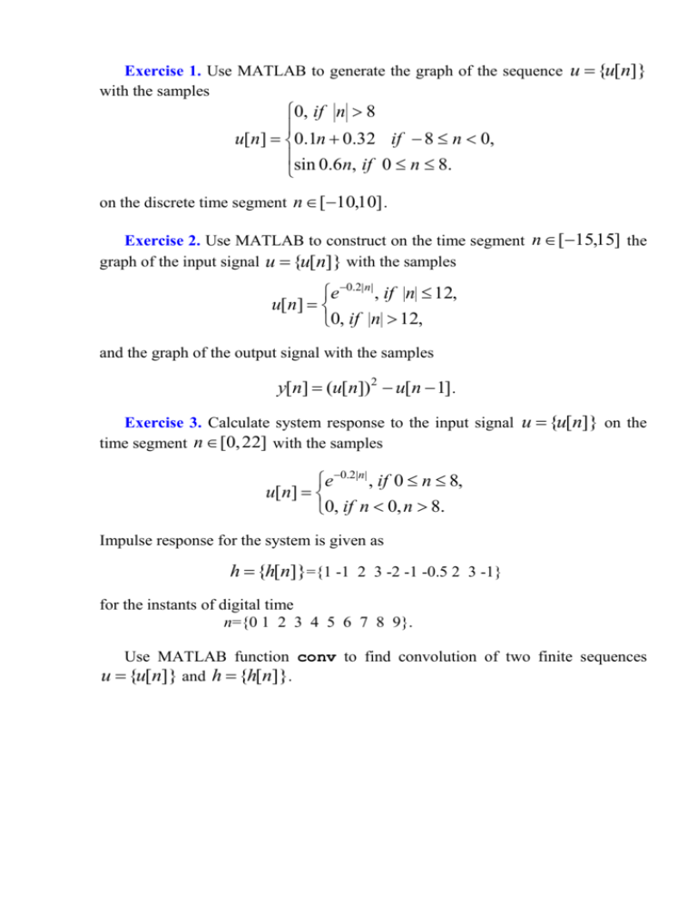
Exercise 1. Use MATLAB to generate the graph of the sequence u  {u[n]}
with the samples
0, if n  8

u[n]  0.1n  0.32 if  8  n  0,
sin 0.6n, if 0  n  8.

on the discrete time segment n  [10,10] .
Exercise 2. Use MATLAB to construct on the time segment n  [15,15] the
graph of the input signal u  {u[n]} with the samples
e 0.2 n , if n  12,
u[n]  
0, if n  12,
and the graph of the output signal with the samples
y[n]  (u[n])2  u[n  1] .
Exercise 3. Calculate system response to the input signal u  {u[n]} on the
time segment n  [0, 22] with the samples
e0.2 n , if 0  n  8,
u[n]  
0, if n  0, n  8.
Impulse response for the system is given as
h  {h[n]}={1 -1 2 3 -2 -1 -0.5 2 3 -1}
for the instants of digital time
n={0 1 2 3 4 5 6 7 8 9}.
Use MATLAB function conv to find convolution of two finite sequences
u  {u[n]} and h  {h[n]}.
Exercise 4. Calculate system response to the input signal u  {u[n]} on the
time segment n  [0, 22] with the samples
e0.2 n , if 0  n  8,
u[n]  
0, if n  0, n  8.
Impulse response for the system is given as
h  {h[n]}={1 -1 2 3 -2 -1 -0.5 2 3 -1}
for the instants of digital time
n={0 1 2 3 4 5 6 7 8 9}.
Use DLTI representation of the system model and the universal function
lsim from the CST package. Repeat the same calculation with the help of the
function filter from DSP-tools.
Exercise 5. Create MATLAB representations as ss, tf and zpk objects for the
following DLTI systems:
x1[n  1]  2 x1[n]  5 x2[n]  2u[n],
a) x2 [ n  1]  3 x1[ n]  2 x2 [ n]  u[ n],
y[n]  2 x1[n]  x2 [n];
 1  2 z 1  3 z  2  3 z 3
u;
b) y 
1  2 z 1  3 z  2  4 z 3  2 z  4
c) zeros: 0.2, –0.1+0.2j, –0.1–0.2j;
poles: 0.3, –0.3+0.1j, –0.3–0.1j, 0.2+0.4j, 0.2–0.4j;
coefficients: 1.
Transform ss-object to tf form, tf-object to ss form and zpk-object to ss form.
Check the eigenvalues of the last ss-object.
Generate random stable discrete-time state-space SISO-model of the 4-th order
and find its transfer function.
Exercise 6. Create MATLAB ss-object in accordance with the following
equations:
x1[n  1]  0.19 x1[n]  0.11x2[n]  0.48x3[n]  0.013x4[n]  0.43u[n],
x2[n  1]  0.11x1[n]  0.46 x2[n]  0.11x3[n]  0.30 x4[n],
x3[n  1]  0.49 x1[n]  0.11x2[n]  0.23x3[n]  0.25x4[n]  0.13u[n],
x4[n  1]  0.013x1[n]  0.30 x2[n]  0.25x3[n]  0.52 x4[n]  0.29u[n],
y[n]  1.2 x2[n]  1.2 x3[n]  0.038x4[n].
Find the transfer function of the created object. Make a linear transformation of
the state vector with the help of non-singular matrix
2  3 2
1


 0  4  2 1
T
3
0
3 1



1

2
1
3


and create the correspondent transformed ss-object. Find its transfer matrix and
compare with the first one.
Generate an impulse response for the above objects with the help of both the
function impulse (CST) and the function impz (DSPT).
Exercise 7. Find magnitude spectrum of the periodic sequence x  x[n]
presented numerically for one period as follows
x p  - 1 - 2 - 1 0 2 3 2 1 2 3 4 5 6 7 6 5.5 4 3.5 4 3
for the instances of discrete time n  0 1 2... 18 19 . Plot this sequence with any
three periods and also plot its magnitude spectrum.
Exercise 8. Analytically obtain Fourier transform for real exponential
sequence f e , given by the formulas
e  n , if n  0;
f e [ n]  
0, if n  0.
Accept   0.3 and plot the correspondent sequence for the signal f e for the
instants of discrete time n  0 1 2... 49 50 . Plot also the graph of this signal
magnitude spectrum for the segment   [20, 20] 1/s of the frequency. In
addition, generate and plot the same magnitude spectrum with the help of the
function fft.
Exercise 9. Plot the frequency response (magnitude and phase) of the DLTI
system, which is represented in the ss form:
x1[n  1]  0.62 x1[n]  0.21x2 [n]  0.08 x3 [n]  0.31u[n],
x2 [n  1]  0.21x1[n]  0.74 x2 [n]  0.05 x3 [n]  0.86u[n],
x3 [n  1]  0.08 x1[n]  0.05 x2 [n]  0.91x3 [n]  0.03u[n],
y[n]  0.16 x1[n]  0.62 x2 [n]  1.09 x3 [n].
Exercise 10. Generate random stable discrete-time state-space SISO-model of
the 5-th order and find its transfer function. Find all the zeros and poles of this
system and plot them on the complex plane with the help of the function zplane
from the DSP-tools. Generate and plot a step response of the obtained DLTI
system.
Generate a priory unstable system with the following zpk-data:
zeros: 0.2, –0.3+0.2j, –0.3–0.2j;
poles: 1.4, –1.2+0.7j, –1.2–0.7j, 0.4+0.3j, 0.4–0.3j;
coefficients: 2.
Plot all the zeros and poles of this system on the complex plane with the help
of the function zplane. Generate and plot a step response of the obtained DLTI
system. Change the poles to 1.8, –1.3+0.7j, –1.3–0.7j, 0.4+0.3j, 0.4–0.3j. Genarate
a step response. Compare with the previous result.
Exercise 11. Consider ss DLTI model
x1[n  1]  0.4 x1[n]  x2 [n]  (1   )u[n],
x2 [n  1]  x1[n],
y[n]  x1[n]  u[n].
Accept the admissible region of parameter  as   [1, 0.5] . Generate and
plot the step response of this system and investigate the dependence of a settling
time and overshoot from the above parameter.
Determin the upper limit for the parameter   0 such that the system is stable.
Exercise 12. For the unstable system with ss-model
x1[n  1]  x2 [n]  u[n],
x2 [n  1]  2 x1[n]  3 x2 [n]  2u[n],
y1[n]  x1[n],
y2 [n]  x2 [n]
design the controller of the form
u[n]  k1x1[n]  k2 x2[n] ,
providing
the
following
eigenvalues of the closed-loop system:
p1  0.2  0.1 j, p2  0.2  0.1 j for various   [0,1] Generate and plot the
correspondent transient process for this system on the variables x2 and u under
initial conditions x1[0]  0 , x2 [0]  10. Investigate a dependence of the process
quality (settling time, overshoot) from the above parameter.
Exercise 13. For the same system as for the previous case with   1 design
the controller of the form
u[n]  k1x1[n]  k2 x2[n] ,
such that the quadratic functional
J  J (K ) 

 x [n]Qx[n]  du [n]Ru[n]
T
T
n 0
achieves its minimum value on the set of stabilizing controllers. Here matrices Q
and R are as follows:
1 0
Q
 , d [0.1, 10] , R  1.
0 1
Generate and plot the transient process of this system on the variables x2 and u
under initial conditions x1[0]  0 , x2 [0]  10.
Investigate a dependence of the process quality (settling time, overshoot) from
the parameter d .