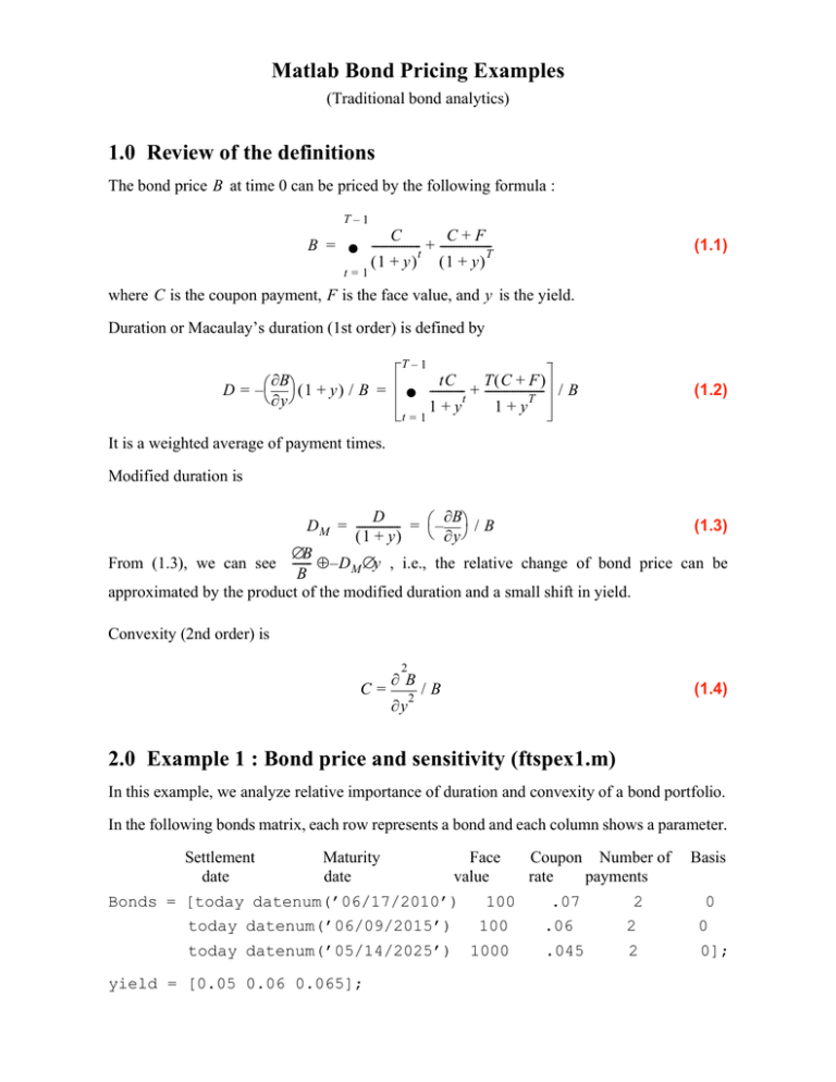
Matlab Bond Pricing Examples
(Traditional bond analytics)
1.0 Review of the definitions
The bond price B at time 0 can be priced by the following formula :
T–1
B =
C
C+F
-t + ------------------T∑ ----------------(1 + y ) (1 + y)
(1.1)
t=1
where C is the coupon payment, F is the face value, and y is the yield.
Duration or Macaulay’s duration (1st order) is defined by
∂B
D = –  ( 1 + y ) / B =
∂y
T–1
tC
T(C + F )
-t + --------------------∑ -----------T
1+y
1+y
/B
(1.2)
t=1
It is a weighted average of payment times.
Modified duration is
D
∂B
D M = ---------------- =  –  / B
(1.3)
( 1 + y)
∂y
∆B
From (1.3), we can see ------- ≈ – D M ∆y , i.e., the relative change of bond price can be
B
approximated by the product of the modified duration and a small shift in yield.
Convexity (2nd order) is
2
C=
∂B
∂y
2
/B
(1.4)
2.0 Example 1 : Bond price and sensitivity (ftspex1.m)
In this example, we analyze relative importance of duration and convexity of a bond portfolio.
In the following bonds matrix, each row represents a bond and each column shows a parameter.
Settlement
Maturity
Face
Coupon Number of
date
date
value
rate
payments
Bonds = [today datenum(’06/17/2010’)
100
.07
2
today datenum(’06/09/2015’)
100
.06
2
today datenum(’05/14/2025’) 1000
.045
2
yield = [0.05 0.06 0.065];
Basis
0
0
0];
Coupon rate is nominal (annual) rate of coupon payments.
prbond is a Matlab function which returns the price p and accrued interest ai of a bond given
all the parameters. The syntax is
[p, ai] = prbond(sd, md, rv, cpn, yld, per, basis)
where sd is the settlement date, md is the maturity date, rv is the par value or face value, cpn
is the coupon rate, yld is the yield, per is the number of coupon periods per year, and the
basis is the day-count basis: 0 = actual/actual, 1 = 30/360, 2 = actual/360, 3 = actual/365.
The coupon rate and number of coupon payments are used to calculate the amount of coupon
C paid during each period. Accrued interest is determined by the following formula :
settlement date – previous coupon date
ai = C ×  ------------------------------------------------------------------------------------------------
time between periods
(2.1)
and the number of days in the numerator and denominator are measured differently according
to the day-count basis.
[d,m] = bonddur(sd, md, rv, cpn, yld, per, basis) finds the Macaulay
duration d and modified duration m in years and [pc,yc] = bondconv(sd, md, rv,
cpn, yld, per, basis) returns the convexity for a security in periods pc and years yc.
The duration of the portfolio p_D M and convexity of the portfolio p_c can be calculated by the
following formula.
3
p_D M =
∑ wi DM (i) and p_c
3
=
i=1
∑ wi yC (i)
(2.2)
i=1
where wi is the the weight of i-th bond in the portfolio and DM(i) and yC(i) are duration and
convexity of i-th bond, respectively.
Suppose there is a shift in yield curve, dY = .002, i.e., 20 basis points where 1 basis point is
1/100 percent or 1/10000.
Percentage change of the portfolio price (linear approximation) is
perc 1 = – p_D M * dY * 100
(2.3)
and the second order approximation is
2
p_c * dY * 100
perc 2 = perc 1 + --------------------------------------2
(2.4)
perc 1 * original
price 1 = original + ------------------------------------100
(2.5)
perc 2 * original
and price 2 = original + ------------------------------------.
100
(2.6)
The approximate prices are
3.0 Example 2 : Hedging against duration and convexity
(ftspex2.m)
This example constructs a bond portfolio to hedge the portfolio of example 1. We assume a long
position in the portfolio in the example 1, and that three other bonds are available for hedging.
We compute weights for these three other bonds in a new portfolio so that the duration and
convexity of the new portfolio match those of the original portfolio.
The following are the bonds we use in hedging :
Settlement
Maturity
Face
Coupon Number of
date
date
value
rate
payments
Bonds = [today datenum(’06/15/2005’)
500
.07
2
today datenum(’08/02/2010’)
today datenum(’03/01/2025’)
1000
250
.066
.08
Basis
0
2
2
0
0];
yield = [0.06 0.07 0.075];
Step 1 : Compute the prices, modified durations - dur1, dur2, and dur3 -, and convexities - conv1,
conv2, and conv3 - of the above bonds using Matlab functions prbond, bonddur, and
bondconv, respectively.
Step 2 : Get the weights of the bonds using the Matlab "\" operator.
dur1
dur2
dur 3
A = conv conv conv and b =
1
2
3
1
1
1
p_D M
p_c
1
(3.1)
and the vector w of weights is
w = A\b
(3.2)
4.0 Example 3 : Visualizing the sensitivity of a bond portfolio’s
price to parallel shifts in the yield curve (ftspex3.m)
This example uses the Financial Toolbox bond pricing functions in a routine that takes time-tomaturity and yield as input arguments and returns the price of a portfolio of bonds. It plots the
price and shows the behavior of bond prices as yield and time vary.
5.0 Yield curves and spot curves from bond data
This example takes coupon bearing bonds with prices as input and generates the following four
graphs.
(1) Extracting yields
Recall
T–1
B =
C
C+F
-t + ------------------T∑ ----------------(1 + y ) (1 + y)
(5.1)
t=1
The Matlab function yldbond returns yields when the bond prices are given. yldbond uses
Newton’t method and cubin spline interpolation.
(2) Spot rate (zero coupon yield curve)
Use bootstrapping and smoothing with splines. Find each successive spot rate by requiring that
the bond of the corresponding maturity be priced correctly, given all the previous rates
calculated. This process is known as the "bootstrapp method" for calculating spot rates.
(3) Extracting a forward rate curve from zero coupon yield curve
Suppose y i and fi are the yield and the forward rate at the time T i respectively. The relation
exp ( y i T i ) = exp ( y i – 1 T i – 1 ) exp ( f i [ T i – T i – 1 ] ) gives the formula for the forward rate.
yi Ti – yi – 1 Ti – 1
fi = -------------------------------------Ti – Ti – 1
(5.2)
6.0 Portfolio Analysis : Heavy use of QPs and LPs
Often finding the optimal portfolio is formulated as a QP.
T
min x Cx
(6.1)
T
s.t. x r ≥ r∗
T
x e = 1
C is a symmetric positive definite (SPD) matrix. The first constraint is for the expected profit.
Variations
(1) If no shorting is allowed, nonnegativity on x is required.
(2) Sometimes there is a disjunctive constraint (much harder) :
x i = 0 or x i ≥ l i > 0
(6.2)
k T
T
min --- x Cx – r x
2
(6.3)
(3) Risk aversion factor
T
x e = 1
where k is the risk tolerance. The objective function is called a utility function.
(4) Downside minimization over scenarios
T
min E ( ( D x – τ )– )
expected gain over benchmark ≥ K
(6.4)
where y_ = min(0, y). The constraint is linear and the optimization problem can be formulates
as LP.
Solving positive definite QPs
1. The problem has a unique global solution.
2. Iterative solution
i) Active set method : finite algorithm
direct matrix factorization
matrix updating
e.g. - Matlab ( to change soon)
- CPLEX
ii) Asymptotic (usually interior)
finds a sequence of points converging to the solution
direct and indirect matrix solutions
fast convergence driven by KT conditions