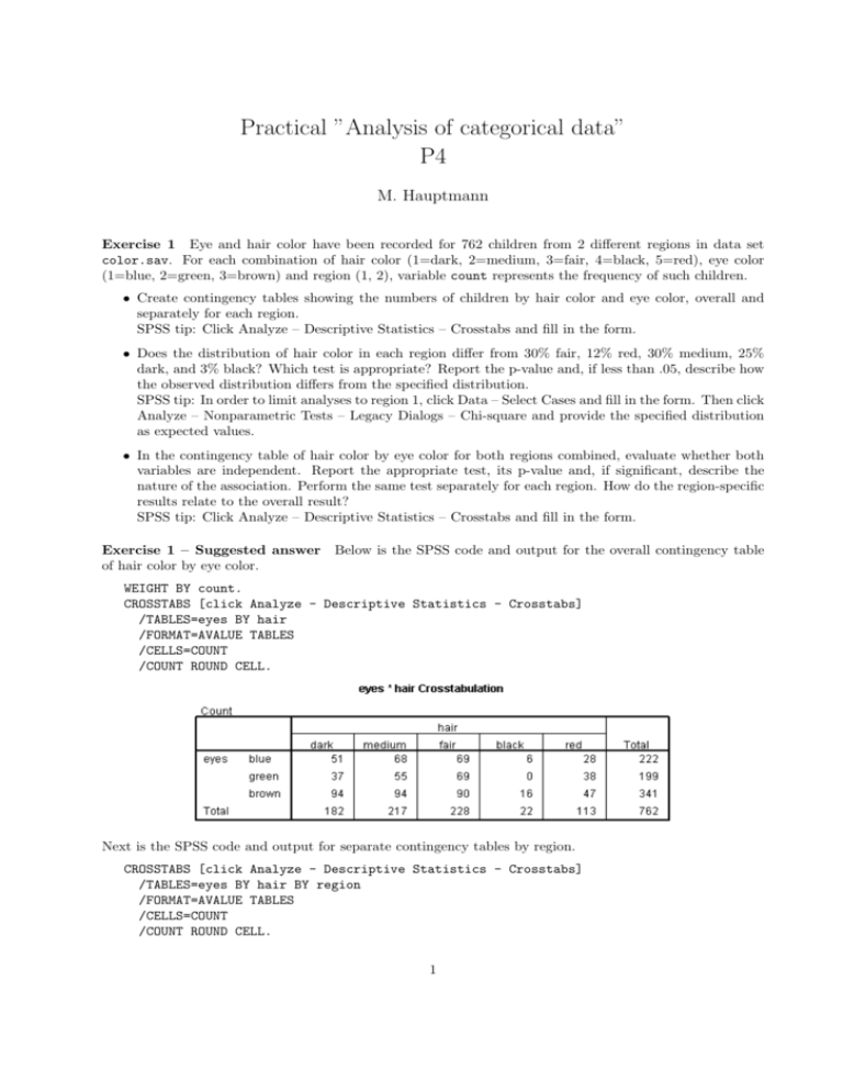
Practical ”Analysis of categorical data”
P4
M. Hauptmann
Exercise 1 Eye and hair color have been recorded for 762 children from 2 different regions in data set
color.sav. For each combination of hair color (1=dark, 2=medium, 3=fair, 4=black, 5=red), eye color
(1=blue, 2=green, 3=brown) and region (1, 2), variable count represents the frequency of such children.
• Create contingency tables showing the numbers of children by hair color and eye color, overall and
separately for each region.
SPSS tip: Click Analyze – Descriptive Statistics – Crosstabs and fill in the form.
• Does the distribution of hair color in each region differ from 30% fair, 12% red, 30% medium, 25%
dark, and 3% black? Which test is appropriate? Report the p-value and, if less than .05, describe how
the observed distribution differs from the specified distribution.
SPSS tip: In order to limit analyses to region 1, click Data – Select Cases and fill in the form. Then click
Analyze – Nonparametric Tests – Legacy Dialogs – Chi-square and provide the specified distribution
as expected values.
• In the contingency table of hair color by eye color for both regions combined, evaluate whether both
variables are independent. Report the appropriate test, its p-value and, if significant, describe the
nature of the association. Perform the same test separately for each region. How do the region-specific
results relate to the overall result?
SPSS tip: Click Analyze – Descriptive Statistics – Crosstabs and fill in the form.
Exercise 1 – Suggested answer Below is the SPSS code and output for the overall contingency table
of hair color by eye color.
WEIGHT BY count.
CROSSTABS [click Analyze - Descriptive Statistics - Crosstabs]
/TABLES=eyes BY hair
/FORMAT=AVALUE TABLES
/CELLS=COUNT
/COUNT ROUND CELL.
Next is the SPSS code and output for separate contingency tables by region.
CROSSTABS [click Analyze - Descriptive Statistics - Crosstabs]
/TABLES=eyes BY hair BY region
/FORMAT=AVALUE TABLES
/CELLS=COUNT
/COUNT ROUND CELL.
1
The appropriate test to compare the observed distribution of hair color with the specified percentages is a
chi-square goodness of fit test. The SPSS code and output for such a test among children from region 1,
including the specification of the expected distribution, is as follows.
USE ALL. [click Data - Select Cases - If and specify region=1]
COMPUTE filter_$=(region=1).
VARIABLE LABEL filter_$ ’region=1 (FILTER)’.
VALUE LABELS filter_$ 0 ’Not Selected’ 1 ’Selected’.
FORMAT filter_$ (f1.0).
FILTER BY filter_$.
EXECUTE.
NPAR TESTS [click Analyze - Nonparametric Tests - Legacy Dialogs - Chi-square]
/CHISQUARE=hair
/EXPECTED=.25 .3 .3 .03 .12 [enter Expected Values]
/MISSING ANALYSIS.
Dito for region=2. The resulting p-values are p=.1008 (region 1) and p=.0003 (region 2), which leads to the
conclusion that the distribution of hair color differed significantly from the hypothesized percentages among
children from region 2, but not among those from region 1.
The appropriate test to evaluate whether hair and eye color are independent is a Pearson chi-square test of
independence. Below is the corresponding SPSS code and output for both regions combined.
2
FILTER OFF.
USE ALL.
EXECUTE.
CROSSTABS [click Analyze - Descriptive Statistics - Crosstabs]
/TABLES=eyes BY hair
/FORMAT=AVALUE TABLES
/STATISTICS=CHISQ [click Statistics - Chi-square]
/CELLS=COUNT
/COUNT ROUND CELL.
There is evidence of an association between eye and hair color (p=0.007). Most of the association is apparently due to more green-eyed children with fair or red hair and fewer such children with dark or black hair.
The opposite occurs among brown-eyed children. Therefore, a child with green eyes has a higher probability
of having fair or red hair, whereas brown-eyed children tend to have dark or black hair more often. The
results by region are p=.125 for region 1 and p=.019 for region 2.
Exercise 2 The mussel data set mussel.sav includes the allele frequencies at the Lap locus in the mussel
Mytilus trossulus on the Oregon coast (McDonald and Siebenaller, Evolution 1989). At four estuaries (variable location), samples were taken from inside the estuary and from marine habitat outside the estuary
(variable habitat). There were 3 common alleles and a couple of rare alleles, here grouped into 94 and non-94
alleles. For each combination of variables, variable count represents the frequency of such observations.
• There is a smaller proportion of 94 alleles in the estuarine location of each estuary when compared
with the marine location – is this difference significant when accounting for location? Which test can
be used to answer the question?
SPSS tip: Click Analyze – Descriptive Statistics – Crosstabs, fill in the form and request the CochranMantel-Haenszel test after clicking on Statistics.
Exercise 2 – Suggested answer The appropriate test is a Cochran-Mantel-Haenszel test and can be
performed with the following SPSS code.
CROSSTABS [click Analyze - Descriptive Statistics - Crosstabs]
/TABLES=habitat BY allele BY location
/FORMAT=AVALUE TABLES
/STATISTICS=RISK CMH(1) [click Statistics - Risk and Cochran-Mantel-Haenszel]
/CELLS=COUNT
/COUNT ROUND CELL.
SPSS first shows the contingency table of habitat by allele stratified for location.
3
In order to get an idea about the strengths of the association within each location, we assess the locationspecific odds ratios between habitat and allele. The association is the strongest in the Tillamook location
(OR=.64) and is around .8 in the other three locations. However, none of the location-specific associations
is statistically significant, as indicated by the fact that all confidence intervals include 1.0. As expected, a
test of homogeneity shows no evidence of heterogeneity (p=.912).
The rest of the output includes the Cochran-Mantel-Haenszel test, which shows significant evidence of an
association between habitat and allele at p=.025, i.e., the null hypothesis that the proportion of Lap94 alleles
is the same in the marine and estuarine locations, accounting for the 4 different locations, can be rejected.
The overall association is OR=.759, i.e., the odds of an allele to be of the 94 type are 24% (=1–.759) lower
in the estuarine habitat compared with the marine habitat.
4
Exercise 3 Data set wheeze.sav contains data on body mass index (BMI, 1=underweight, 2=normal,
3=overweight, 4=obese) and wheezing after exercise (0=no, 1=yes) from a cross-sectional survey among
4,010 children aged 13–14 yrs in Brazil (Cassol et al., Jornal de Pediatria 2005). Variable count indicates
the frequency of observations.
• Does the prevalence of wheezing differ between the 4 BMI groups? Does the prevalence of wheezing
increase with increasing BMI group? Which tests answer those questions?
SPSS tip: Click Analyze – Descriptive Statistics – Crosstabs, fill in the form and request Chi-square
after clicking on Statistics.
Exercise 3 – Suggested answer The following SPSS code prepares a contingency table of BMI by
wheezing and performs a Pearson chi-square test as well as a linear-by-linear association test.
WEIGHT BY count.
CROSSTABS [click Analyze - Descriptive Statistics - Crosstabs]
/TABLES=bmi BY wheeze
/FORMAT=AVALUE TABLES
/STATISTICS=CHISQ [click Statistics - Chi-square]
/CELLS=COUNT ROW
/COUNT ROUND CELL.
5
The output shows that there is no significant evidence of an association when the Pearson chi-square test
is used (p=.064), which treats variable BMI as a nominal variable (no order). When the linear-by-linear
association test is used with scores 1, 2, 3, 4 representing the order of categorical variable BMI, the p-value
becomes significant (p=.011), i.e., there is significant evidence of a trend in wheezing prevalence with BMI
(generally increasing or decreasing, in this case increasing). The example shows that the linear-by-linear
association test has more statistical power than the Pearson chi-square test for the evaluation of ordered
variables against alternatives of monotone trend.
Exercise 4 Richard Feynman, member of the presidential commission to investigate the explosion of the
Challenger space shuttle, suspected that the low temperature at take-off caused the O-rings to fail. The
space-shuttle O-ring data set oring.sav contains data on temperature and O-ring failures from 24 previous
space shuttle flights (Feynmann: Why do we care what other people think, 1988).
• How much evidence do those data provide for Feynman’s hypothesis? Perform a Kruskal-Wallis test
and describe the results.
SPSS tip: Click Analyze – Nonparametric Tests – Legacy Dialogs – K Independent Samples, fill in the
form and make sure the Kruskal-Wallis test is requested.
• Alternatively, one could perform a linear-by-linear association test with the number of O-ring incidents
as row scores and take-off temperatures as column scores. Compare the result of this test with a
standard Pearson chi-square test which ignores the ordering. Which test is more powerful?
SPSS tip: Click Analyze – Descriptive Statistics – Crosstabs, fill in the form and request Chi-square
after clicking on Statistics.
Exercise 4 – Suggested answer The following SPSS code requests a Kruskal-Wallis test for temperature
by the number of O-ring failures. An exact p-value based on Monte Carlo simulation is requested because
the sample size is too small for the asymptotics of the test to work reliably.
NPAR TESTS [click Analyze - Nonparametric Tests - Legacy Dialogs - Chi-square]
/K-W=temp BY oring(0 3)
/MISSING ANALYSIS
/METHOD=MC CIN(99) SAMPLES(10000). [click Exact - Monte Carlo]
6
The Kruskal-Wallis test provides evidence that the median temperature differs by the number of O-ring
incidents (p=.016). The mean rank for each number of O-ring failures also indicates heterogeneity (note
that the Kruskal-Wallis test is a rank test based on the ranks rather than the actually observed values of the
outcome variable). However, the number of O-ring failures is considered nominal, therefore ignoring that
there is actually an order (e.g., 3 failures are more than 2).
SPSS code and output for Pearson chi-square and linear-by-linear association tests is given below.
CROSSTABS [click Analyze - Descriptive Statistics - Crosstabs]
/TABLES=oring BY temp
/FORMAT=AVALUE TABLES
/STATISTICS=CHISQ [click Statistics - Chi-square]
/CELLS=COUNT
/COUNT ROUND CELL
/METHOD=MC CIN(99) SAMPLES(10000). [click Exact - Monte Carlo]
The results show that the Pearson chi-square test does not reject independence (p=.270, note the large
number of degrees of freedom) whereas the linear-by-linear association test (1 degree of freedom) does
(p=.005). The latter is not ignoring the ordering of the number of O-ring incidents but exploits the ordinal
scale of the number of O-ring incidents and evaluates whether there is an increasing or decreasing trend in
the temperature with the number of O-ring incidents. The test is therefore more powerful against trend
alternatives. The negative sign of the standardized test statistic (-2.698) suggests an inverse association, i.e.,
the number of O-ring incidents is increasing with decreasing temperature at take-off.
Exercise 5 The drug toxicity data set drugtox.sav includes data on patients treated with 4 doses of a
drug (in mg) and 4 degrees of toxicity: 1=mild, 2=moderate, 3=severe, and 4=drug death (Hoyle: Statistical
strategies for small sample research 1999). Variable count indicates the frequency of patients for a given
dose and toxicity.
• Make a table of toxicity by dose group and describe the observed data. Which tests are appropriate
for evaluating a possible association between drug dose and toxicity? Perform those and interpret the
results. Note that data outside the mild toxicity category are sparse and it therefore appears prudent
to request exact p-values based on Monte Carlo simulations.
SPSS tip: Click Analyze – Descriptive Statistics – Crosstabs, fill in the form and request Chi-square
after clicking on Statistics. Also, click Exact and request Monte Carlo or Exact.
• Someone makes the case that drug death should be considered catastrophic and orders of magnitude
more serious than severe toxicity and suggests to use a score of 10,000 for drug death. Perform the test
again with the modified score for the highest category. How do the results differ from the standard
scores 1, 2, 3, 4?
SPSS tip: Create a new variable with 10,000 as the maximum value by clicking Transform – Compute
Variable, fill in the form and run the Chi-square test as above on the new variable.
Exercise 5 – Suggested answer In this example, ordinal toxicity categories are the outcome and data
are grouped by 4 ordinal categories of dose. A table can be produced by the following SPSS code.
WEIGHT BY count.
CROSSTABS [click Analyze - Descriptive Statistics - Crosstabs]
/TABLES=dose BY tox
7
/FORMAT=AVALUE TABLES
/CELLS=COUNT
/COUNT ROUND CELL.
Only few of the 226 subjects in the study have any toxicity, making inference difficult. However, it appears
that higher degrees of toxicity only occurred among subjects in higher dose groups. The only toxicity-related
death occurred among subjects in the highest dose category.
In order to exploit the ordinal nature of both variables, we can use the linear-by-linear association test.
SPSS code and output are given below.
CROSSTABS [click Analyze - Descriptive Statistics - Crosstabs]
/TABLES=dose BY tox
/FORMAT=AVALUE TABLES
/STATISTICS=CHISQ [click Statistics - Chi-square]
/CELLS=COUNT
/COUNT ROUND CELL
/METHOD=EXACT TIMER(2). [click Exact - Exact]
Although the positive sign of the standardized test statistic indicates toxicity is increasing with increasing
dose (1.744), the evidence is not statistically significant (p=.091).
SPSS code and output is provided below for repeating the linear-by-linear association test with a modified
score for the highest toxicity category, i.e. for scores 1, 2, 3, 10,000 instead of equally spaced scores 1, 2, 3,
4.
COMPUTE tox_new=tox*(tox<4)+10000*(tox=4). EXECUTE. [click Transform - Compute Variable]
CROSSTABS [click Analyze - Descriptive Statistics - Crosstabs]
/TABLES=dose BY tox_new
/FORMAT=AVALUE TABLES
/STATISTICS=CHISQ [click Statistics - Chi-square]
/CELLS=COUNT
/COUNT ROUND CELL
/METHOD=EXACT TIMER(2). [click Exact - Exact]
8
With the modified scores, the test now provides significant evidence that higher doses are associated with
higher degrees of toxicity (p=.042).
Exercise 6 The cytomegalovirus data set cmv.sav contains data on a comparison of formaldehyde and
acetone fixations for the cytomegalovirus antigenemia assay. Variables AC_detected and FA_detected indicate whether CMV was detected (0=no, 1=yes) by acetone (AC) and formaldehyde (FA), respectively.
Variable count indicates the frequency of samples per group. In 405 samples, cytomegalovirus was detected
36 times (8.8%) using formaldehyde and 22 times (5.4%) using acetone (Perez et al., J Clin Microbiol 1995).
Acetone
Detected
Not detected
Formaldehyde
Detected
Not detected
18
4
18
365
36/405=8.8%
369
22/405=5.4%
383
405
• Evaluate whether the proportion of detection is significantly greater for formaldehyde compared with
acetone. Which test is appropriate?
SPSS tip: Tell SPSS about the frequency with which each record occurred by clicking Data – Weight
Cases and selecting the appropriate variable. Then click Analyze – Descriptive Statistics – Crosstabs,
fill in the form and make sure McNemar is requested after clicking on Statistics.
• Calculate McNemar’s test using the formula presented in the lecture, which only uses the numbers of
discordant pairs.
Exercise 6 – Suggested answer Under the null hypothesis that both fixations are equally efficient,
we would expect that discrepancies are split 50/50. However, the probability that a discrepancy favors
formaldehyde is actually 82% (18/22). The SPSS code below performs McNemar’s test.
WEIGHT BY count. [click Data - Weight Cases]
CROSSTABS [click Analyze - Descriptive Statistics - Crosstabs]
/TABLES=AC_detected BY FA_detected
/FORMAT=AVALUE TABLES
/STATISTICS=MCNEMAR [click Statistics - McNemar]
/CELLS=COUNT
/COUNT ROUND CELL.
9
The output shows that the difference is statistically significant at p=.004. McNemar’s test ignores the 18
times that both tests detect CMV and the 365 times that neither test detected CMV – these are noninformative data. Only discordant pairs provide information about a possible discrepancy between the
proportions. This becomes obvious when applying the formula presented in the lecture,
χ2 =
(|b − c| − 1)2
b+c
The chi-square statistic can be calculated as (|18-4|-1)2 /(18+4) at 1 DF, which results in a p-value of .0056.
The slight difference is due to the continuity correction.
An alternative analysis would be to calculate a 95% confidence interval around the proportion that a discrepancy favors formaldehyde, i.e., 18/22=82% (95% CI: 67–98). Because 50% is not included in the confidence
interval, there is significant evidence that the proportion of detection is significantly greater for formaldehyde
compared with acetone.
10