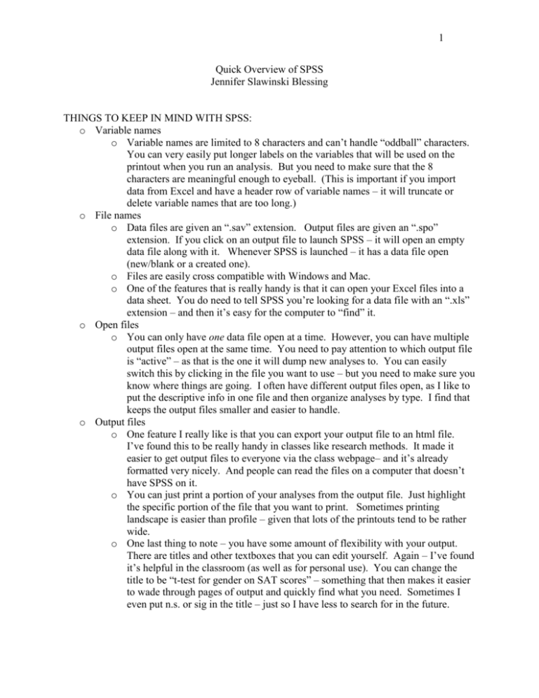
1
Quick Overview of SPSS
Jennifer Slawinski Blessing
THINGS TO KEEP IN MIND WITH SPSS:
o Variable names
o Variable names are limited to 8 characters and can’t handle “oddball” characters.
You can very easily put longer labels on the variables that will be used on the
printout when you run an analysis. But you need to make sure that the 8
characters are meaningful enough to eyeball. (This is important if you import
data from Excel and have a header row of variable names – it will truncate or
delete variable names that are too long.)
o File names
o Data files are given an “.sav” extension. Output files are given an “.spo”
extension. If you click on an output file to launch SPSS – it will open an empty
data file along with it. Whenever SPSS is launched – it has a data file open
(new/blank or a created one).
o Files are easily cross compatible with Windows and Mac.
o One of the features that is really handy is that it can open your Excel files into a
data sheet. You do need to tell SPSS you’re looking for a data file with an “.xls”
extension – and then it’s easy for the computer to “find” it.
o Open files
o You can only have one data file open at a time. However, you can have multiple
output files open at the same time. You need to pay attention to which output file
is “active” – as that is the one it will dump new analyses to. You can easily
switch this by clicking in the file you want to use – but you need to make sure you
know where things are going. I often have different output files open, as I like to
put the descriptive info in one file and then organize analyses by type. I find that
keeps the output files smaller and easier to handle.
o Output files
o One feature I really like is that you can export your output file to an html file.
I’ve found this to be really handy in classes like research methods. It made it
easier to get output files to everyone via the class webpage– and it’s already
formatted very nicely. And people can read the files on a computer that doesn’t
have SPSS on it.
o You can just print a portion of your analyses from the output file. Just highlight
the specific portion of the file that you want to print. Sometimes printing
landscape is easier than profile – given that lots of the printouts tend to be rather
wide.
o One last thing to note – you have some amount of flexibility with your output.
There are titles and other textboxes that you can edit yourself. Again – I’ve found
it’s helpful in the classroom (as well as for personal use). You can change the
title to be “t-test for gender on SAT scores” – something that then makes it easier
to wade through pages of output and quickly find what you need. Sometimes I
even put n.s. or sig in the title – just so I have less to search for in the future.
2

FILE
o As with any software – this is the go to place for opening and saving files. You
can open any data or output file from here. To get an Excel sheet open – just go
to “open” and make sure to select the correct extension (.xls) for the computer to
search for.
o Also – under “save as” you can save your data file as an Excel file.
o
o DATA
o Some useful commands here:
 “Sort cases” – I often have to do this to find discrepant data points within a
variable. You can sort on more than one variable (like Excel). To unsort –
you need to have a variable of case numbers to sort along.
 “Select Cases” – The default is that SPSS selects all the cases to use. But you
can set up a conditional for it to choose, or select random cases, or based on a
range or some key variable. You then have the option to delete the
“unselected” cases or have them just filtered. I often will just filter them –
and then you can go back and reset it back to all cases.
3
TRANSFORM
o The two most useful tools here are “Compute” and “Recode”
o Compute is helpful in creating aggregate scores, averages, etc. It will create a new
variable and then you need to “plug in” the formula under “numeric expression”.
There is a list of functions – or you can type in your own formula.
o You can see in the screenshot that the list of all variables is listed on the left – and
you can add them to your formula by selecting them and clicking the gray arrow
button. (If they are categorical or string variables – they will not be available in the
list.)
4
o With recode – you can recode into the same variable (i.e. change your codes). Can be
handy if you made a mistake or what to use different groupings.
o You can also recode into a new variable. So – I’ve used this to do things like retain a
variable of “grade in school” but then create a new variable of “school” – primary,
middle, high, etc.
5
o
o ANALYZE
o This is the heart of where all the fun stuff happens. I’ll just try to make a short
guideline of key types of analyses and where you can find them.
o Key things under DESCRIPTIVE STATISTICS
o Frequencies
o Descriptive stats
o Crosstabs – the easiest way to run a Chi-square is to use this one.
 **Chi-square is also available under the “Nonparametric Tests” – but it
only can handle one variable – it cannot do a two variable analysis.
o Key things under COMPARE MEANS
o One sample t-test
o Independent samples t-test
o Paired samples t-test
o One-way ANOVA
6
o Key things under General Linear Model
o Univariate
o Multivariate
o Repeated Measures
o Key things under Correlate
o Bivariate
o Partial
o On many of the means comparisons – you want to make sure to click “descriptive stats”
(under options) otherwise the printout on the output file will NOT include means – just
the F-tests, etc.
7
o Data Entry
o
Look for this in lower left corner of data sheet. Or
double click on a variable name to get to “variable view”
In variable view – you describe your variable. The default settings are probably the ones you
want – (type=numeric, columns = 8, 2 decimal places, no missing values etc).
Important things:
Use the “LABEL” to come up with less truncated names for the variables – these labels will print
out on your output
Use “VALUES” to set value assignments – such as 1=male, 2= female. This assignment makes
ANOVAs and T-tests much easier to compute rather than using the words as your values.
o
8
Crosstabs & Chi-square
The only way to do a Chi-square between two categorical variables is to compute a “Crosstabs”
which is under descriptive statistics
o When you click on “Crosstabs” you’ll see the following options:
o You want to select variables from the left column and “send” them to the appropriate
label (Row or column).
o To get the Chi-square – click on “STATISTICS” and select Chi-square
o
o You also might want to have it report the expected values and percentages for the cells.
To do so – click on “Cells” and it will give you the options for that.
o An output of what crosstabs with a chi-square looks like follows:
o
9
Case Proce ssing S ummary
Cases
Valid
N
Gender * M inority
Classification
M issing
Percent
474
N
100.0%
Total
Percent
0
N
Percent
.0%
Gender * Min ority Classification Crosstabulation
Count
M inority
Classification
Gender
No
194
male
female
Yes
Total
64
176
40
Total
Chi-S quare Tests
Pearson Chi-Square
Continuity Correction
Likelihood Ratio
1
Asymp. Sig.
(2-sided)
.099
2.359
1
.125
2.738
1
.098
Value
2.714
a
df
b
Exact Sig.
(2-sided)
Fisher's Exact Test
.119
Linear-by-Linear
Association
2.708
N of Valid Cases
474
1
.100
a. Comp uted only for a 2x2 table
b. 0 cells (.0%) have expected count less than 5. The minimum expected count is
47.39.
Exact Sig.
(1-sided)
10
o T-test
o
o You have three options for T-tests: one-sample, independent-samples, and pairedsamples. All of them conduct a 2-tailed test – so keep that in mind.
o I’ll use an example of an independent-samples:
o
o As with the crosstabs (and all analyses)– you have all your variables lined up on the left –
and you need to select and send them to the right place. You can run t-tests on more than
one DEPENDENT variable at the same time – provided you want to use the same
grouping variable.
o IMPORTANT NOTE: you can run t-tests even if you have 3 or more groups. You
MUST (even with 2 groups) define which levels of your INDEPENDENT variable you
want to use. So when you assign a “grouping variable” – you then will need to define
groups “1” and “2” - or “3” and “6” – or whatever your values are. This is why it’s
important to assign values to labels (such as 1=male).
Below is an example printout
TTEST Output
11
Group S tatistics
Current Salary
Gender
male
N
258
M ean
******
Std.
Deviation
********
Std. Error
M ean
female
Indepen de nt S amples Te st
Levene's Test for
Equality of
Variances
F
Current Salary
Equal variances
assumed
119.67
Sig.
.000
t-test for Equality of M eans
t
10.945
df
472
Sig.
(2-tailed)
.000
M ean
Difference
Std. Error
Difference
95% Confidence
Interval of the
Difference
Lower
Upper
$15,409.86
Equal variances
not assumed
o ANOVA
o You can simply find a simple one-way ANOVA under the same “Compare Means” –
where you find a t-test. The box looks like this:
o
o
o An important thing to know – YOU ALWAYS want to go to “options” and check that
you want the descriptive stats….otherwise it will give you the F-test but NO means or
standard deviations for your groups.
o
12
o You can also do two-way (and more) ANOVAs – found under “GENERAL LINEAR
MODEL”
o
o The box for the Univariate ANOVA is as follows:
o
o
o
o Again – you have to click on options and “Descriptive stats” in order to get means printed
out. With this option – you can only test one DEPENDENT variable at a time. With the
the one-way ANOVA option – you can run several ANOVAs on several DEPENDENT
variables at once – much like the t-tests. It is an efficient way of getting analyses done –
if appropriate for your project.
o
13
o Multiple Regression
o Can be found at:
o
14
Repeated Measures
o
15
o Creating Categorical variables out of continuous ones (or binning the variable)
SPSS can be asked to create any number of categories for a particular variable. Find it here:
The popup menu is easy and look as follows: