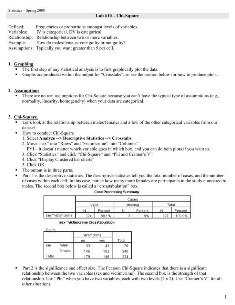
Statistics – Spring 2008
Lab #10 – Chi-Square
Defined:
Variables:
Relationship:
Example:
Assumptions:
Frequencies or proportions amongst levels of variables.
IV is categorical, DV is categorical
Relationship between two or more variables.
How do males/females vote guilty or not guilty?
Typically you want greater than 5 per cell.
1. Graphing
 The first step of any statistical analysis is to first graphically plot the data.
 Graphs are produced within the output for “Crosstabs”, so see the section below for how to produce plots.
2. Assumptions
 There are no real assumptions for Chi-Square because you can’t have the typical type of assumptions (e.g.,
normality, linearity, homogeneity) when your data are categorical.
3. Chi-Square.
 Let’s look at the relationship between males/females and a few of the other categorical variables from our
dataset.
 How to conduct Chi-Square
1. Select Analyze --> Descriptive Statistics --> Crosstabs
2. Move “sex” into “Rows” and “victimcrime” into “Columns”
FYI – it doesn’t matter which variable goes in which box, and you can do both plots if you want to.
3. Click “Statistics” and click “Chi-Square” and “Phi and Cramer’s V”.
4. Click “Display Clustered bar charts”
5. Click OK.
 The output is in three parts.
 Part 1 is the descriptive statistics. The descriptive statistics tell you the total number of cases, and the number
of cases within each cell. In this case, notice how many more females are participants in the study compared to
males. The second box below is called a “crosstabulation” box.

Part 2 is the significance and effect size. The Pearson Chi-Square indicates that there is a significant
relationship between the two variables (sex and victimcrime). The second box is the strength of that
relationship. Use “Phi” when you have two variables, each with two levels (2 x 2). Use “Cramer’s V” for all
other situations.
1

Part 3 is the chart.
2


WRITE-UP. The information included in the write up is the chi-square value, df, and significance value.
Lately the field as a whole has recommended that you report effect size as well.
a. There was a significant relationship between males/females and whether or not they were victims of a
crime, χ2(1) = 5.6, p = .018. Males were significantly more likely to be a victim of crime than females.
The effect size was .132.
EVALUATION. You want to look at three pieces of information: (1) is the effect significant (p-value), (2)
what is the size of the effect (effect size), and (3) what is the direction of the effect (the count within each cell.
4. Chi-Square (another example)
 Let’s look at the relationship between voter (republican, democrat, none, other) and the “death_threelevels”
variable we created in a previous lab where 1=support death penalty, 2=neutral, and 3=oppose death penalty.
 This example is a 4 x 3.
 When you move beyond just testing a 2 x 2, then the output in SPSS for the crosstabs analysis is treated as an
“Omnibus” test, similar to the Omnibus test in ANOVA, in which you treat the Omnibus test as telling you
whether one or more of the follow-up tests are significant. If the Omnibus test is significant, then you conduct
follow-up tests of the multiple 2 x 2 relationships within the larger combinations (in this case, 4 x 3).
 How to conduct Chi-Square
1. Select Analyze --> Descriptive Statistics --> Crosstabs
2. Move “voter” into “Rows” and “death_threelevels” into “Columns”
FYI – it doesn’t matter which variable goes in which box, and you can do both plots if you want to.
3. Click “Statistics” and click “Chi-Square” and “Phi and Cramer’s V”.
4. Click “Display Clustered bar charts”
5. Click OK.
 The output is in three parts.
 Part 1 is the descriptive statistics. The descriptive statistics tell you the total number of cases, and the number
of cases within each cell.
3

Part 2 is the significance and effect size. The Pearson Chi-Square indicates that there is a significant
relationship amongst the variables. The second box is the strength of that relationship. Use “Phi” when you
have two variables, each with two levels (2 x 2). Use “Cramer’s V” for all other situations.

Part 3 is the chart.
4










Follow-up tests:
You can conduct all possible 2 x 2 relationships within the larger combination (4 x 3).
I am going to show you an example of one of the possible follow-up tests.
From the chart above, it looks like one of the more interesting relationships is between Republicans and
Democrats because they are equal in the neutral condition and are polarized in opposite directions in the
“support the death penalty” and “oppose the death penalty” conditions.
Thus, let’s test a 2 x 2 for Republican/Democrat and Support/Oppose.
First, you use “select cases” to restrict which cases SPSS will analyze. Second, you conduct the same
crosstabs analysis as before, but this time SPSS will only analyze the data you have indicated via “select
cases”.
For example, to select cases:
1. Select Data --> Select Cases”.
2. Click “If condition is satisfied”, then click “If..”
3. In the open box, type --> voter <= 2 & death_threelevels ~= 2
FYI – This text tells SPSS to restrict analysis for the “voter” variable to only levels below 2, and to restrict
analysis for the “death_threelevels” variable to any level except 2.
4. Click “Continue”
5. Click OK.
Now, repeat the “crosstabs” analysis just as before, without changing anything.
1. Select Analyze --> Descriptive Statistics --> Crosstabs
2. Move “voter” into “Rows” and “death_threelevels” into “Columns”
FYI – it doesn’t matter which variable goes in which box, and you can do both plots if you want to.
3. Click “Statistics” and click “Chi-Square” and “Phi and Cramer’s V”.
4. Click “Display Clustered bar charts”
5. Click OK.
The output is in three parts.
Part 1 is the descriptive statistics. The descriptive statistics tell you the total number of cases, and the number
of cases within each cell.
Part 2 is the significance and effect size. The Pearson Chi-Square indicates that there is a significant
relationship amongst the variables. The second box is the strength of that relationship. Use “Phi” when you
have two variables, each with two levels (2 x 2). Use “Cramer’s V” for all other situations.
5

Part 3 is the chart.

WRITE-UP. The information included in the write up is the chi-square value, df, and significance value.
Lately the field as a whole has recommended that you report effect size as well.
a. There was a significant relationship between the two variables , χ2(6) = 29.68, p < .001. A follow-up
test between Republican/Democrats and support/oppose the death penalty found that Republicans were
significantly more likely to support the death penalty and Democrats were significantly more likely to
oppose the death penalty, χ2(1) = 22.54, p < .001. The effect size was .367.
EVALUATION. You want to look at three pieces of information: (1) is the effect significant (p-value), (2)
what is the size of the effect (effect size), and (3) what is the direction of the effect (the count within each cell.

6