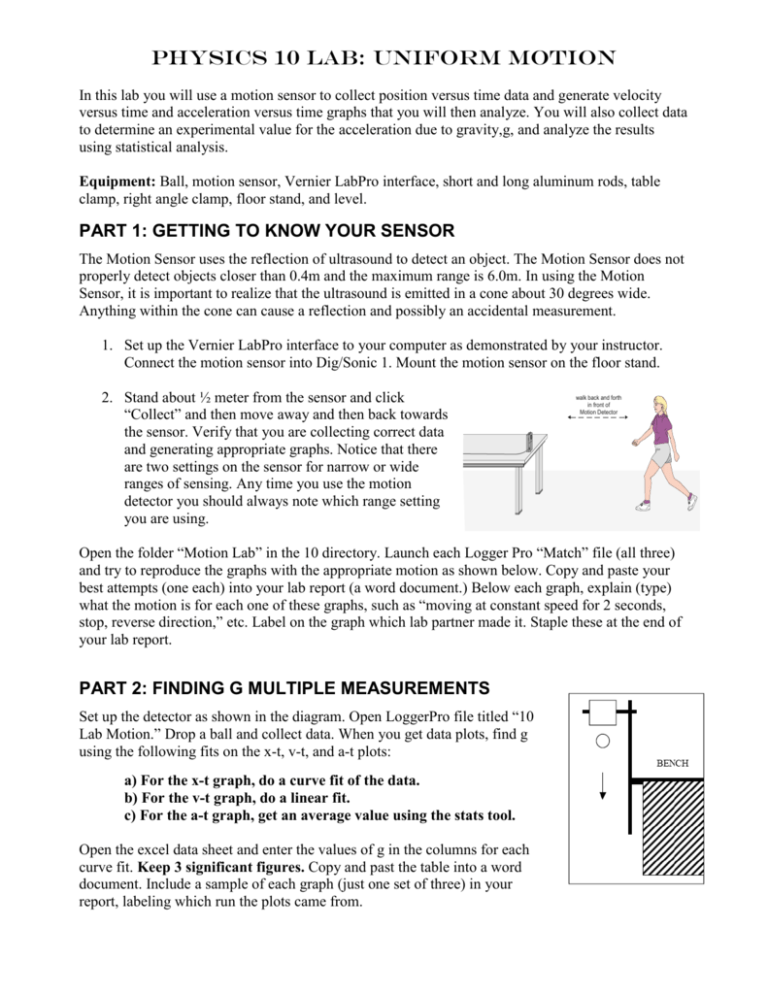
Physics 10 Lab: Uniform Motion
In this lab you will use a motion sensor to collect position versus time data and generate velocity
versus time and acceleration versus time graphs that you will then analyze. You will also collect data
to determine an experimental value for the acceleration due to gravity,g, and analyze the results
using statistical analysis.
Equipment: Ball, motion sensor, Vernier LabPro interface, short and long aluminum rods, table
clamp, right angle clamp, floor stand, and level.
PART 1: GETTING TO KNOW YOUR SENSOR
The Motion Sensor uses the reflection of ultrasound to detect an object. The Motion Sensor does not
properly detect objects closer than 0.4m and the maximum range is 6.0m. In using the Motion
Sensor, it is important to realize that the ultrasound is emitted in a cone about 30 degrees wide.
Anything within the cone can cause a reflection and possibly an accidental measurement.
1. Set up the Vernier LabPro interface to your computer as demonstrated by your instructor.
Connect the motion sensor into Dig/Sonic 1. Mount the motion sensor on the floor stand.
2. Stand about ½ meter from the sensor and click
“Collect” and then move away and then back towards
the sensor. Verify that you are collecting correct data
and generating appropriate graphs. Notice that there
are two settings on the sensor for narrow or wide
ranges of sensing. Any time you use the motion
detector you should always note which range setting
you are using.
walk back and forth
in front of
Motion Detector
Open the folder “Motion Lab” in the 10 directory. Launch each Logger Pro “Match” file (all three)
and try to reproduce the graphs with the appropriate motion as shown below. Copy and paste your
best attempts (one each) into your lab report (a word document.) Below each graph, explain (type)
what the motion is for each one of these graphs, such as “moving at constant speed for 2 seconds,
stop, reverse direction,” etc. Label on the graph which lab partner made it. Staple these at the end of
your lab report.
PART 2: FINDING G MULTIPLE MEASUREMENTS
Set up the detector as shown in the diagram. Open LoggerPro file titled “10
Lab Motion.” Drop a ball and collect data. When you get data plots, find g
using the following fits on the x-t, v-t, and a-t plots:
a) For the x-t graph, do a curve fit of the data.
b) For the v-t graph, do a linear fit.
c) For the a-t graph, get an average value using the stats tool.
Open the excel data sheet and enter the values of g in the columns for each
curve fit. Keep 3 significant figures. Copy and past the table into a word
document. Include a sample of each graph (just one set of three) in your
report, labeling which run the plots came from.
PART 2 CON’T: ANALYSIS OF THE DATA
In Excel, find the average value and average deviation of each for each set of data for the x-t, v-t and
a-t columns. Express your final values for g in ‘standard form’ using the average value as your final
g and the standard deviation as your uncertainty. Box these. Label them. You should have three.
Taking 9.80m/s^2 as the ‘true’ value of g, use Excel to find the discrepancy and % discrepancy for
each set of data. Also, express your discrepancy as a multiple of your uncertainty and use the table
below to determine the quality of the experimental agreement, that is, how well the results agree
with the probability of a normal distribution. Then you can express your final results using all this
information. Here is a sample:
The experimental value of g (8.6+/-0.5)m/s^2 from the x-t data is off from the accepted value of
9.8 m/s^2 by 1.2 m/s^2, 12.2%, which is a discrepancy of 2.4 sigmas, which is fair agreement.
Type a conclusion summarizing your results. Be sure to include the following, keeping it as
concise and thorough as possible:
1. What was the goal of your experiment? What method did you use?
2. What assumptions did you make and how do you predict this will effect your results (make them
higher, lower, etc.)?
3. What were your results (expressed with uncertainty) for each x-t, v-t and a-t plot?
4. What is the accepted value you are comparing it to?
5. Compare your results to the accepted value using discrepancy, percent discrepancy, discrepancy in
terms of sigma and quality of agreement.
6. Which plot gave you the best agreement? For which plots did the true value fall within the range
of experimental values.