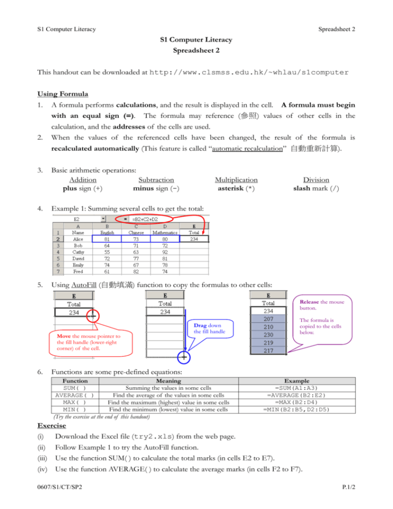
S1 Computer Literacy
Spreadsheet 2
S1 Computer Literacy
Spreadsheet 2
This handout can be downloaded at http://www.clsmss.edu.hk/~whlau/s1computer
Using Formula
1. A formula performs calculations, and the result is displayed in the cell. A formula must begin
with an equal sign (=). The formula may reference (參照) values of other cells in the
calculation, and the addresses of the cells are used.
2. When the values of the referenced cells have been changed, the result of the formula is
recalculated automatically (This feature is called “automatic recalculation” 自動重新計算).
3.
Basic arithmetic operations:
Addition
Subtraction
plus sign (+)
minus sign (-)
Multiplication
asterisk (*)
Division
slash mark (/)
4.
Example 1: Summing several cells to get the total:
5.
Using AutoFill (自動填滿) function to copy the formulas to other cells:
Release the mouse
button.
Move the mouse pointer to
the fill handle (lower-right
corner) of the cell.
6.
Drag down
the fill handle
The formula is
copied to the cells
below.
Functions are some pre-defined equations:
Function
Meaning
SUM( )
Summing the values in some cells
AVERAGE( )
Find the average of the values in some cells
MAX( )
Find the maximum (highest) value in some cells
MIN( )
Find the minimum (lowest) value in some cells
(Try the exercise at the end of this handout)
Example
=SUM(A1:A3)
=AVERAGE(B2:E2)
=MAX(B2:D4)
=MIN(B2:B5,D2:D5)
Exercise
(i)
(ii)
(iii)
(iv)
Download the Excel file (try2.xls) from the web page.
Follow Example 1 to try the AutoFill function.
Use the function SUM( ) to calculate the total marks (in cells E2 to E7).
Use the function AVERAGE( ) to calculate the average marks (in cells F2 to F7).
0607/S1/CT/SP2
P.1/2
S1 Computer Literacy
Spreadsheet 2
Relative Address (相對位址) and Absolute Address (絶對位址)
7. When a formula is copied, the addresses in the formula are changed automatically. They are
relative addresses. In the example of step 4-5, the formula in E2 is “=B2+C2+D2”, and when it
is copied to the E3, the formula is changed to be “=B3+C3+D3” automatically.
8.
If an address should be fixed (固定) when it is copied, we should use absolute address. A dollar
sign ($) should be added before the row number and/or column letter in the address.
9.
Example 2: Calculating an overall mark.
a)
When we use the AutoFill to copy the formula from D2 the cells below:
What’s wrong? Let’s check the formula in D3 and D6.
b) In order to fix the row numbers in the addresses G3 and G4, a dollar sign ($) should be
inserted before the row numbers, and the formula in D2 become “=B2*G$3+C2*G$4”.
c)
Now repeat AutoFill again, correct results are shown:
10. We may use absolute address in cell range too. For example, we may add a
column to find out the rank (排名) of the students. We use the
function RANK( value , cell_range )in cell E2.
Type here:
=RANK( D2 , D$2:D$7 )
Exercise
(v) Follow your teacher’s demonstration and work on Example 2 using the file try2.xls.
Reference
http://www.usd.edu/trio/tut/excel/
http://www.baycongroup.com/el0.htm
http://www.utexas.edu/its/training/handouts/UTOPIA_ExcelGS/
0607/S1/CT/SP2
P.2/2