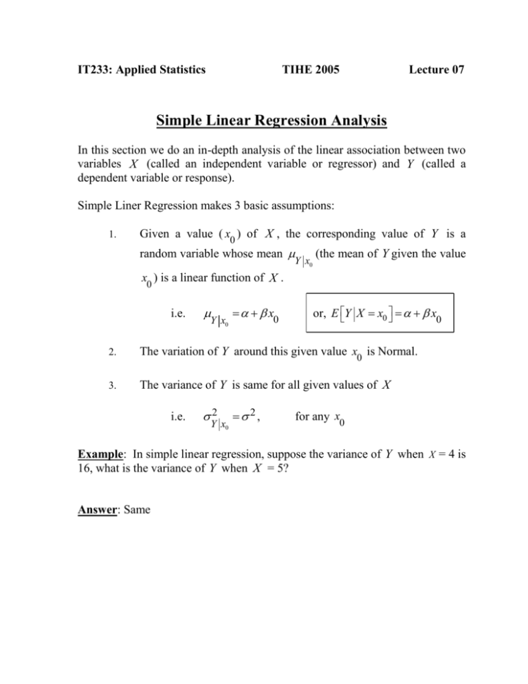
IT233: Applied Statistics
TIHE 2005
Lecture 07
Simple Linear Regression Analysis
In this section we do an in-depth analysis of the linear association between two
variables X (called an independent variable or regressor) and Y (called a
dependent variable or response).
Simple Liner Regression makes 3 basic assumptions:
1.
Given a value ( x0 ) of X , the corresponding value of Y is a
random variable whose mean 
(the mean of Y given the value
Y x0
x0 ) is a linear function of X .
i.e.

Y x0
    x0
or, E Y X  x0      x0
2.
The variation of Y around this given value x0 is Normal.
3.
The variance of Y is same for all given values of X
i.e.
2
Y x0
 2 ,
for any x0
Example: In simple linear regression, suppose the variance of Y when X = 4 is
16, what is the variance of Y when X = 5?
Answer: Same
Simple Linear Regression Model:
Using the above assumptions, we can write the model as:
Y    x 
Where  is a random variable (or error term) and follows normal distribution
with E ( )  0 and Var ( )   2
i.e.


N 0,  2

Illustration of Linear Regression:
Let X = the height of father
Y = the height of son
For fathers whose height is x0 , the heights of the sons will vary randomly.
Linear regression states that the height on son is a linear function of the height
of father i.e.
Y    x
Scatter Diagrams:
A scatter diagram will suggest whether a simple linear regression model would
be a good fit.
Figure (A) suggests that a simple linear regression model seems OK, though
the fit is not very good (Wide scatter around the fitted lines).
Figure (B) suggest that a simple linear regression model seems to fit well
(points are closed to the fitted line).
In (C) a straight line could be fitted, but relationship is not linear.
In (D) there is no relationship between Y and X .
Fitting a Linear Regression Equation:
Keep in mind that there are two lines
Y
Y     x (True line)
Yˆ  ˆ  ˆ x (Estimated line)
X
Notation:
a (or ˆ ) = Estimate of 
b (or ˆ ) = Estimate of 
yi
= The observed value of Y corresponding to xi
yˆ
= The fitted value of Y corresponding to xi
i
ei
= y  yˆ = The residual .
i
i
Residual: The error in Fit:
The residual, denoted by ei = y  yˆ , is the difference between the observed
i
i
and fitted values of Y . It estimates i .
Y
yi
Yˆ  ˆ  ˆ x

ei 

yˆ i
xi
X
The Method of Least Squares:
We shall find a (or ˆ ) and b (or ˆ ) , the estimates of  and  , so that the sum
of the squares of the residuals is minimum. The residual sum of squares is often
called the sum of squares of the errors about the regression line and denoted by
SSE . This minimization procedure for estimating the parameters is called the
method of least squares. Hence, we shall find a and b so as to minimize
n

i 1
n
SSE   ei2   yi  yˆi
i 1

2

i 1
n
  yi  a  bxi

2
Differentiating SSE with respect to a and b and setting the partial derivatives
equal to zero, we obtain the equations (called the normal equations).
n
n
i 1
i 1
n
n
n
i 1
i 1
i 1
na  b  xi   yi
a  xi  b  xi2   xi yi
Which may be solved simultaneously for a and b .