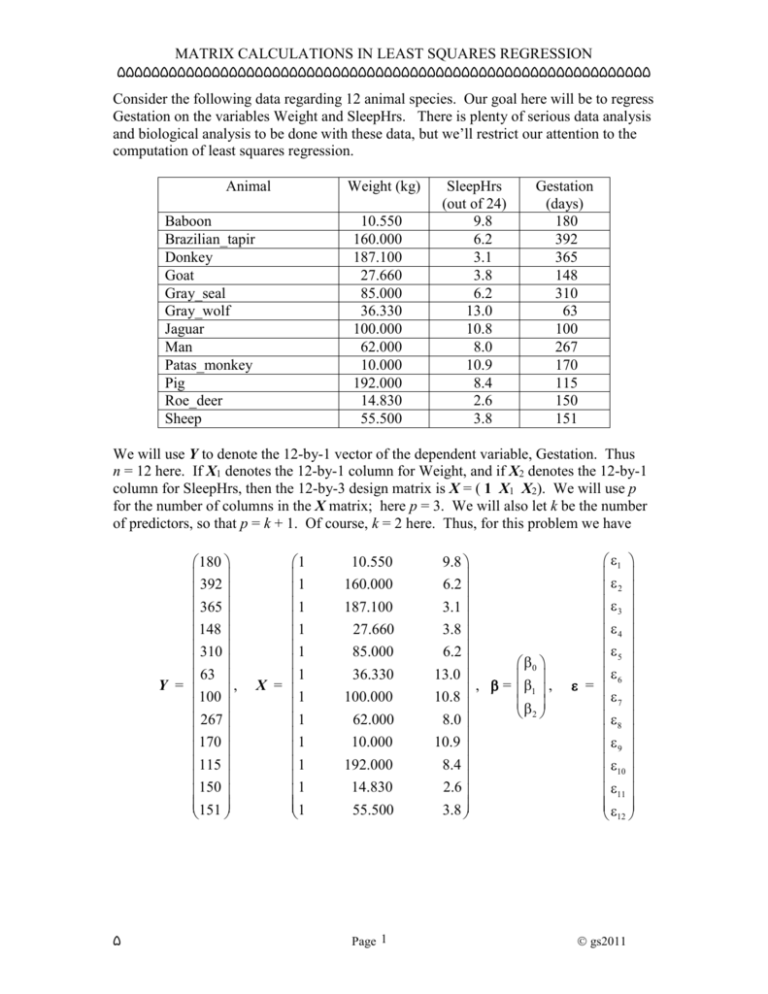
MATRIX CALCULATIONS IN LEAST SQUARES REGRESSION
۵۵۵۵۵۵۵۵۵۵۵۵۵۵۵۵۵۵۵۵۵۵۵۵۵۵۵۵۵۵۵۵۵۵۵۵۵۵۵۵۵۵۵۵۵۵۵۵۵۵۵۵۵۵۵۵۵۵۵۵۵۵
Consider the following data regarding 12 animal species. Our goal here will be to regress
Gestation on the variables Weight and SleepHrs. There is plenty of serious data analysis
and biological analysis to be done with these data, but we’ll restrict our attention to the
computation of least squares regression.
Animal
Baboon
Brazilian_tapir
Donkey
Goat
Gray_seal
Gray_wolf
Jaguar
Man
Patas_monkey
Pig
Roe_deer
Sheep
Weight (kg)
10.550
160.000
187.100
27.660
85.000
36.330
100.000
62.000
10.000
192.000
14.830
55.500
SleepHrs
(out of 24)
9.8
6.2
3.1
3.8
6.2
13.0
10.8
8.0
10.9
8.4
2.6
3.8
Gestation
(days)
180
392
365
148
310
63
100
267
170
115
150
151
We will use Y to denote the 12-by-1 vector of the dependent variable, Gestation. Thus
n = 12 here. If X1 denotes the 12-by-1 column for Weight, and if X2 denotes the 12-by-1
column for SleepHrs, then the 12-by-3 design matrix is X = ( 1 X1 X2). We will use p
for the number of columns in the X matrix; here p = 3. We will also let k be the number
of predictors, so that p = k + 1. Of course, k = 2 here. Thus, for this problem we have
 180 


 392 
 365 


 148 
 310 


 63 
Y = 
,
100 


 267 
 170 


 115 


 150 
 151 
۵
1

1
1

1
1

1
X = 
1

1
1

1

1
1
10.550
160.000
187.100
27.660
85.000
36.330
100.000
62.000
10.000
192.000
14.830
55.500
Page 1
9.8 

6.2 
3.1 

3.8 
6.2 

13.0 
, =
10.8 

8.0 
10.9 
8.4 

2.6 
3.8 
 0 
 
 1  ,
 
 2
 1 
 
 2 
 3 
 
 4 
 
 5 
 6 
 =  
 7 
 8 
 
 9 
 10 
 
 11 
 
 12 
 gs2011
MATRIX CALCULATIONS IN LEAST SQUARES REGRESSION
۵۵۵۵۵۵۵۵۵۵۵۵۵۵۵۵۵۵۵۵۵۵۵۵۵۵۵۵۵۵۵۵۵۵۵۵۵۵۵۵۵۵۵۵۵۵۵۵۵۵۵۵۵۵۵۵۵۵۵۵۵۵
The linear regression model is Y = X  + . The first task in a regression is usually the
estimation of . This is done through setting up the normal equations, which should be
solved for b, the estimate for . The normal equations here are the 3-by-3 system
(X X) b = X  Y
If the matrix X X is non-singular (which is usually the case), then we can actually solve
this system in the form b = (X X)-1 X  Y . Here we have
941.0
86.6 
 12.0


X X =  941.0 124,135.8 6,327.1 
 86.6
6,327.1
757.2 

How did we get this? In terms of its columns, we wrote X = ( 1 X1 X2). Therefore, the
1 X1
1 X 2 
 11
 1 


 
transpose is X  =  X1  , leading to X X =  X1 1 X1 X1 X1 X 2  . Each entry is the


 X 
 X 1 X  X X  X 
 2
2
1
2
2
 2
simple inner product of two n-by-1 vectors. For example, the entry X  X refers to the
1
2
arithmetic
10.55  9.8 + 160.00  6.2 + 187.10  3.1 + ….
+ 55.50  3.8  6,327.1
Inversion of the 3-by-3 matrix X X can be done by a number of methods. Page 12 of
Draper and Smith actually shows the algebraic form of the inverse of a 3-by-3 matrix.
Let us note for the record that it is rather messy to invert a 3-by-3 matrix. The actual
inverse (found by Minitab) is
(X X)
-1
 0.698018 0.002129 0.062046 


=  0.002129 0.000021 0.000072 
 0.062046 0.000072 0.007816 


Just for comparison, the inverse found by S-Plus is
(X X)-1
 0.698017814 0.00212866891 0.06204619519 


=  0.002128669 0.00002052342 0.00007196429 
 0.062046192 0.00007196429 0.00781568202 


It seems simply that S-Plus has reported more figures.
۵
Page 2
 gs2011
MATRIX CALCULATIONS IN LEAST SQUARES REGRESSION
۵۵۵۵۵۵۵۵۵۵۵۵۵۵۵۵۵۵۵۵۵۵۵۵۵۵۵۵۵۵۵۵۵۵۵۵۵۵۵۵۵۵۵۵۵۵۵۵۵۵۵۵۵۵۵۵۵۵۵۵۵۵
Now let’s note that X Y is the 3-by-1 vector
 2, 411
 1 Y 




X Y = X1 Y =  226,582 


 15, 628 
 X Y 


 2 
This leads finally to
b = (X X)-1 X  Y
 0.698018 0.002129 0.062046 


=  0.002129 0.000021 0.000072 
 0.062046 0.000072 0.007816 


 2, 411
 230.939 




 226,582  =  0.643 
 15, 628 
 11.143 




These were obtained with Minitab. This means that the fitted regression equation is
Y = 230.939 + 0.643 X1 - 11.143 X2
This could be expressed with the actual variable names
ˆ
= 230.939 + 0.643 Weight - 11.143 SleepHrs
Gestation
The fitted vector is Yˆ , computed as Yˆ = X b = X (X X)-1 X Y.
It’s very convenient to use the symbol H = X (X X)-1 X . We’ll note later that this is the
n-by-n projection matrix into the linear space spanned by the columns of X. This allows
us to write Yˆ = H Y .
The matrix H is sometimes called the “hat” matrix because it is used to produce
the fitted vector Yˆ (“y-hat”). As this is the projection into the linear space of the
columns of X, it is sometimes written as PX .
There is considerable interest in the n-by-n matrix H. For this situation, H is this:
0.204781 -0.030694 -0.110852 0.092290
-0.030694 0.216082 0.265908 0.009151
-0.110852 0.265908 0.393823 0.068363
0.092290 0.009151 0.068363 0.252397
0.059823 0.095988 0.120832 0.105716
0.222648 0.003947 -0.138914 -0.038041
0.112131 0.110464 0.037823 -0.053235
0.115134 0.055425 0.032506 0.080688
0.222282 -0.033857 -0.138704 0.059607
-0.035640 0.262758 0.274230 -0.098833
0.089407 -0.008903 0.072769 0.305344
0.058690 0.053730 0.122216 0.216553
۵
0.059823
0.095988
0.120832
0.105716
0.091338
0.037511
0.057897
0.076463
0.051570
0.081534
0.113887
0.107442
0.222648 0.112131
0.003947 0.110464
-0.138914 0.037823
-0.038041 -0.053235
0.037511 0.057897
0.346062 0.224790
0.224790 0.204384
0.123714 0.094984
0.269284 0.144261
0.082405 0.197923
-0.082906 -0.097699
-0.050500 -0.033722
Page 3
0.115134 0.222282 -0.035640 0.089407 0.058690
0.055425 -0.033857 0.262758 -0.008903 0.053730
0.032506 -0.138704 0.274230 0.072769 0.122216
0.080688 0.059607 -0.098833 0.305344 0.216553
0.076463 0.051570 0.081534 0.113887 0.107442
0.123714 0.269284 0.082405 -0.082906 -0.050500
0.094984 0.144261 0.197923 -0.097699 -0.033722
0.091808 0.120723 0.057319 0.078358 0.072879
0.120723 0.249159 -0.017804 0.045583 0.027896
0.057319 -0.017804 0.378411 -0.150742 -0.031562
0.078358 0.045583 -0.150742 0.375139 0.259764
0.072879 0.027896 -0.031562 0.259764 0.196615
 gs2011
MATRIX CALCULATIONS IN LEAST SQUARES REGRESSION
۵۵۵۵۵۵۵۵۵۵۵۵۵۵۵۵۵۵۵۵۵۵۵۵۵۵۵۵۵۵۵۵۵۵۵۵۵۵۵۵۵۵۵۵۵۵۵۵۵۵۵۵۵۵۵۵۵۵۵۵۵۵
The small print is necessary to display this 12-by-12 matrix. The diagonal entries are
called the leverage values, and these are shown here in bold type.
We should note this interesting property for H :
HH =H
This is easily verified, as H H = [ X (X X)-1 X  ] [ X (X X)-1 X  ]
1
1
= X (X X)-1 X  X (X X)-1 X  = X  X  X  X  X  X  X  X 
This product is the identity I .
= X (X X) I X  = X (X X) X  = H .
-1
-1
A matrix with property AA = A is called idempotent. It is easily verified that I - H is
also idempotent.
The analysis of variance centers about the equation
Y  Y = Y  ( I - H + H ) Y = Y  ( I - H) Y + Y  H Y
This is a right-triangle type of relationship. We can identify the component parts:
YY
YHY
Y  ( I - H) Y
Total sum of squares (not corrected for the mean) with n
degrees of freedom.
Regression sum of squares (not corrected for the mean)
with p degrees of freedom.
Error (or residual) sum of squares with n - p degrees of
freedom.
These can be summarized in the following analysis of variance framework:
Source of
Variation
Regression
Error (Residual)
Total
Degrees of
Freedom
p
n-p
n
Sum Squares
YHY = bXY
Y  ( I - H) Y = Y  Y – b  X  Y
YY
This is given without the columns for Mean Squares and F. We’ll use these in the more
useful table (which corrects for the mean) coming later.
The alternate form for the regression sum of squares comes from Y  H Y
1
= Y  X  X  X  X  Y = b  X  Y. The alternate form for the error sum of squares is
This is b
similarly derived.
۵
Page 4
 gs2011
MATRIX CALCULATIONS IN LEAST SQUARES REGRESSION
۵۵۵۵۵۵۵۵۵۵۵۵۵۵۵۵۵۵۵۵۵۵۵۵۵۵۵۵۵۵۵۵۵۵۵۵۵۵۵۵۵۵۵۵۵۵۵۵۵۵۵۵۵۵۵۵۵۵۵۵۵۵
The more useful version of the analysis of variance is done with the correction for the
mean.
Our model can be written in coordinate form as
Gestationi = 0 + W Weighti + S SleepHrsi + i
There seems to be no possibility of confusion in shortening the names if we use G for
Gestation, W for Weight, and S for SleepHrs. Thus, we’ll write this as
Gi = 0 + W Wi + S Si + i
Let W be the average value of the weights, and let S be the average of the sleep hours
variable. We can write the above as
Gi = (0 + W W + S S ) + W (Wi - W ) + S (Si - S ) + i
Using
*
symbols to note quantities which have been revised, write this as
Gi = *0 + W Wi * + S S i* + i
We will call this the mean-centered form of the model. Indeed, all our computations will
use the mean-centered form.
Note that the coefficients W and S have not changed. The new intercept *0 is related to
0 through *0 = 0 + W W + S S . This means that we can fit the mean-centered form
of the model and then recover 0, as 0 = *0 - W W - S S .
In matrix form, the mean-centered form is Y = X*  * + . We have noted that
 *0

* =  W
 S

۵

 0  W W   S S 



W
 = 




S



Page 5
 gs2011
MATRIX CALCULATIONS IN LEAST SQUARES REGRESSION
۵۵۵۵۵۵۵۵۵۵۵۵۵۵۵۵۵۵۵۵۵۵۵۵۵۵۵۵۵۵۵۵۵۵۵۵۵۵۵۵۵۵۵۵۵۵۵۵۵۵۵۵۵۵۵۵۵۵۵۵۵۵
Here is the mean-centered matrix X* :
2.5833333 
 1 67.864167


81.585833 1.0166667 
1
 1 108.685833 4.1166667 


 1 50.754167 3.4166667 
1
6.585833 1.0166667 


1

42.084167
4.7833333


X* = 
1
21.585833
3.5833333 


0.7833333 
 1 16.414167
 1 68.414167
3.6833333 

 1 113.585833
1.1833333 


 1 63.584167 4.6166667 
 1 22.914167 3.4166667 


The second and third columns have means of zero. This leads to a very useful
consequence:
(X*) 
12

X =  0
 0

*


50,350.46
463.6108 
463.6108 132.2167 
0
0
This was computed by S-Plus. In fact, the zeroes in positions
(1, 2) and (2, 1) were computed as -9.947598  10-14. The zeroes
in positions (1, 3) and (3, 1) were computed as -8.881784  10-15.
The least squares solution requires the inversion of (X*)  X* . However, the
computational complexity is that of a two-by-two inversion! This is so much easier than
a three-by-three inversion. See the illustrations on page 121 of Draper and Smith.
The computational complexity of a p-by-p inversion is
proportional to p3. For this problem, we see that a problem of
complexity 33 = 27 has been reduced to complexity 23 = 8. This is
an impressive saving. In a problem with p = 5 (four predictors)
we can reduce the complexity from 53 = 125 to 43 = 64.
We can give also the mean-centered version of the analysis of variance table. This
logically involves the centering of Y. That is, we write Y = Y* + Y 1 , where Y* is the
vector with the mean removed. For these data,
۵
Page 6
 gs2011
MATRIX CALCULATIONS IN LEAST SQUARES REGRESSION
۵۵۵۵۵۵۵۵۵۵۵۵۵۵۵۵۵۵۵۵۵۵۵۵۵۵۵۵۵۵۵۵۵۵۵۵۵۵۵۵۵۵۵۵۵۵۵۵۵۵۵۵۵۵۵۵۵۵۵۵۵۵
 -20.91667

 191.08333
 164.08333

 -52.91667
 109.08333

 -137.91667
*
Y = 
-100.91667

 66.08333
 -30.91667

 -85.91667

 -50.91667
 -49.91667




















1
1 1 , which is sometimes called the
n
1
1
mean sweeper. The diagonal entries are 1  , and the off-diagonal entries are  . It
n
n
1


follows that Y* =  I  1 1  Y .
n


You can actually describe this with the matrix I -
Now observe that Y*  1 = 0, as the entries of Y* sum to zero. Then
Y  Y = (Y* + Y 1) (Y* + Y 1) = Y*  Y* + Y 1 Y* + Y Y*  1 + Y 2 1 1
= Y*  Y* + 0 + 0 + n Y 2
In coordinate form, this says
n
Y
i 1
n
2
i
=
 Y  Y 
i 1
i
2
+ n Y2
These can be identified further:
YY
Y*  Y*
n Y2
۵
Total sum of squares (not corrected for the mean) with n
degrees of freedom.
Total sum of squares (corrected for the mean) with n - 1
degrees of freedom, often called SYY
Sum of squares for the mean with 1 degree of freedom,
often called CF for “correction factor”
Page 7
 gs2011
MATRIX CALCULATIONS IN LEAST SQUARES REGRESSION
۵۵۵۵۵۵۵۵۵۵۵۵۵۵۵۵۵۵۵۵۵۵۵۵۵۵۵۵۵۵۵۵۵۵۵۵۵۵۵۵۵۵۵۵۵۵۵۵۵۵۵۵۵۵۵۵۵۵۵۵۵۵
This leads us to the common form of the analysis of variance table:
Source of
Variation
Regression
(corrected
for b0)
Degrees of
Freedom
Error
(Residual)
Total
(corrected)
Sum Squares
Mean Squares
F
k
Y  H Y - n Y2
= b X  Y - n Y 2
Y  H Y  nY 2
k
MS(Regression)
MS  Error 
n-k-1
Y  ( I - H) Y
= Y  Y - b X  Y
Y     H Y
n-1
Y  Y - n Y 2 = SYY
n2
Recall that X is n-by-p, and it includes the column 1. Here p = k + 1, where k is the
number of predictors.
Sum Square
. In
Degrees of Freedom
Mean Square (Regression)
the regression analysis of variance table, F =
.
Mean Square (Error)
In general, in any analysis of variance table, Mean Square =
The vector Yˆ = H Y is the fitted vector. Also, e = (I - H) Y is the residual vector.
This says also that Y = Yˆ - e. The error sum of squares is e  e.
Using the matrix notation, you can show the following:
e  Yˆ = 0
The residual and fitted vectors are orthogonal.
If c is a column of X , then
Hc = c
This follows from H X = X.
H1=1
This is a special case of the above.
e1=0
The residuals sum to zero.
Y  1 = Yˆ  1
The average Y-value is the same as the average fitted value.
H e= 0
۵
Page 8
 gs2011
MATRIX CALCULATIONS IN LEAST SQUARES REGRESSION
۵۵۵۵۵۵۵۵۵۵۵۵۵۵۵۵۵۵۵۵۵۵۵۵۵۵۵۵۵۵۵۵۵۵۵۵۵۵۵۵۵۵۵۵۵۵۵۵۵۵۵۵۵۵۵۵۵۵۵۵۵۵
For the case in which there is one predictor, we can use the second version on page 131
of Draper and Smith. Remember, this is the form specific for the situation in which
there is one predictor.
Source of
Variation
Regression
SS(b1| b0)
Error
(Residual)
Total
(corrected)
Degrees of
Freedom
Sum Squares
Mean Squares
1
Y  H Y - n Y2
= b X  Y - n Y 2
Y  H Y - n Y2
= b X  Y - n Y 2
n-2
Y  ( I - H) Y
= Y  Y - b X  Y
Y     H Y
n-1
Y  Y - n Y 2 = SYY
F
b X Y  nY 2
Y     H Y
n2
n2
For this problem with one predictor, you might find these computing forms useful:
Source of
Variation
Degrees of
Freedom
Regression
1
Error
Mean Squares
 S XY 
 S XY 
2
S XX
SYY -
n-2
Total
Sum of Squares
 S XY 
MS Regression
MS Error
S XX
2
SYY 
 S XY 
2
S XX
n2
S XX
n-1
2
F
SYY
This uses these formulas:
n
SXX =
 Xi  X  =
2
i 1
 X
n
SXY =
i 1
n
SYY =
X
i 1
2
i
2
i
i  X  Yi  Y  =
- n X2
n
XY
i 1
i i
- nX Y
n
 by  y g=  Y
i 1
۵
n
i 1
i
2
- n Y2
Page 9
 gs2011