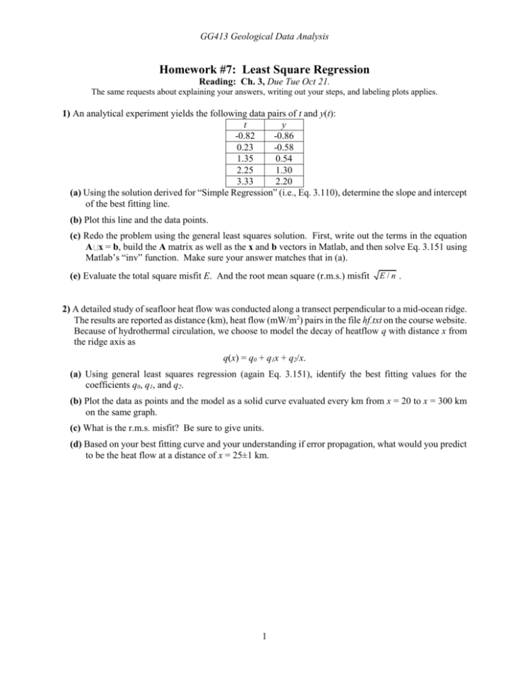
GG413 Geological Data Analysis
Homework #7: Least Square Regression
Reading: Ch. 3, Due Tue Oct 21.
The same requests about explaining your answers, writing out your steps, and labeling plots applies.
1) An analytical experiment yields the following data pairs of t and y(t):
t
y
-0.82
-0.86
0.23
-0.58
1.35
0.54
2.25
1.30
3.33
2.20
(a) Using the solution derived for “Simple Regression” (i.e., Eq. 3.110), determine the slope and intercept
of the best fitting line.
(b) Plot this line and the data points.
(c) Redo the problem using the general least squares solution. First, write out the terms in the equation
A x = b, build the A matrix as well as the x and b vectors in Matlab, and then solve Eq. 3.151 using
Matlab’s “inv” function. Make sure your answer matches that in (a).
(e) Evaluate the total square misfit E. And the root mean square (r.m.s.) misfit
E/n .
2) A detailed study of seafloor heat flow was conducted along a transect perpendicular to a mid-ocean ridge.
The results are reported as distance (km), heat flow (mW/m2) pairs in the file hf.txt on the course website.
Because of hydrothermal circulation, we choose to model the decay of heatflow q with distance x from
the ridge axis as
q(x) = q0 + q1x + q2/x.
(a) Using general least squares regression (again Eq. 3.151), identify the best fitting values for the
coefficients q0, q1, and q2.
(b) Plot the data as points and the model as a solid curve evaluated every km from x = 20 to x = 300 km
on the same graph.
(c) What is the r.m.s. misfit? Be sure to give units.
(d) Based on your best fitting curve and your understanding if error propagation, what would you predict
to be the heat flow at a distance of x = 25±1 km.
1