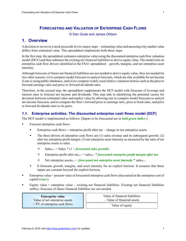
Forecasting and Valuation of Enterprise Cash Flows
1
FORECASTING AND VALUATION OF ENTERPRISE CASH FLOWS
© Dan Gode and James Ohlson
1. Overview
A decision to invest in a stock proceeds in two major steps – estimating value and assessing why market value
differs from estimated value. This spreadsheet implements both these steps.
In the first step, the spreadsheet estimates enterprise value using the discounted enterprise cash flow valuation
model (DCF) and then subtracts the existing net financial liabilities to derive equity value. The model rests on
enterprise cash flow drivers identified in the FSA1 spreadsheet – growth, margins, and net enterprise asset
intensity.
Although forecasts of future net financial liabilities are not needed to derive equity value, they are needed for
two other reasons: (i) to compare model forecasts to analyst forecasts, which are only available for net income
if one is using public databases, and (ii) to compute widely used relative valuation metrics such as the price to
forward earnings ratio and price to forward dividends ratio.
Therefore, in the second step, the spreadsheet supplements the DCF model with forecasts of leverage and
interest rates to forecast net income and dividends. This step aids in identifying the potential causes for
deviation between estimated value and market value by allowing one to compare model forecasts to analyst
net income forecasts, and to compare the firm’s forward price to earnings ratio, price to book ratio, and price
to forward dividends ratio to its peers.
Enterprise activities: The discounted enterprise cash flows model (DCF)
1.1.
The DCF model is implemented as follows: [Inputs to be forecasted are in bold green italics.]

Forecast enterprise cash flows

Enterprise cash flows = enterprise profit after tax – change in net enterprise assets

The three drivers of enterprise cash flows are (1) sales revenue and its subsequent growth; (2)
after tax enterprise profit margin; (3) net enterprise asset intensity as measured by the ratio of net
enterprise assets to sales.


Salest+1 = Salest * (1 + forecasted sales growth)

Enterprise profit after taxt+1 = salest+1 * forecasted enterprise profit margin after tax

Net enterprise assetst+1 = forecasted net enterprise asset intensity * salest+1
It forecasts growth, margins, and asset intensity for an explicit horizon. It assumes that these
inputs are constant beyond the explicit horizon.

Enterprise value = present value of forecasted enterprise cash flows discounted at the enterprise cost of
capital (wacc).

Equity value = enterprise value – existing net financial liabilities. Existing net financial liabilities
suffice; forecasts of future financial liabilities are not needed.
Enterprise value
Value of net enterprise assets
= PV of enterprise cash flows
February 9, 2016 Visit http://www.godeohlson.com/ for updates.
Value of financial liabilities
– Value of financial assets
Value of equity
1
Forecasting and Valuation of Enterprise Cash Flows
2
Financial activities: Net income, dividends, and book value of equity
1.2.
This part of the spreadsheet proceeds as follows:

Derive financial statements

Net financial liabilities = forecasted ratio of net financial liabilities to net enterprise assets * net
enterprise assets

Net financial expense after tax = forecasted net financial expense rate after tax * net financial
liabilities

Net income = enterprise profit after tax – net financial expense after tax

Net distributions = contributions from equity holders – distributions to equity holders = enterprise
cash flows – net financial expense after tax + change in net financial liabilities

Ending equity = Beginning equity + net income – net distributions

Check: Equity = Net enterprise assets – Net financial liabilities

Derive relative valuation metrics: It computes three key relative valuation metrics: price to book ratio,
price to forward earnings ratio, and price to forward dividends ratio.

Infer cost of equity: If one uses a subjective wacc or industry wacc, then it is useful to know the cost of
equity implied by the assumed wacc and estimated value. Accordingly, the spreadsheet infers the cost of
equity from wacc and leverage so that it can be compared with alternative measures of cost of equity.
Enterprise cost of capital or weighted-average cost of capital (wacc)
1.3.
The spreadsheet needs wacc as an input to discount enterprise cash flows. The spreadsheet does not specify
how wacc should be derived. One can use industry wacc or a subjective measure of wacc.
Textbooks derive wacc using a company’s equity beta, leverage, and risk-free rate as follows:
wacc =
MV of NFL * Net interest rate, after tax
MV of NFL + MV of E
+
MV of E * re
MV of NFL + MV of E
This expression is the genesis of the term wacc because it is the weighted average of re and cost of NFL. This
expression provides a way of inferring wacc from re and cost of NFL.
The weighted average formula applies to negative leverage as well. The net interest rate after tax should be
the interest rate on net financial assets after tax. When this rate is close to zero, the first term in the wacc
formula drops out and the wacc formula reduces to the following:
wacc =
MV of equity
MV of equity - NFA
x re
As a practical matter, one can estimate wacc as follows:
1.
Go to the latest balance sheet and derive NFL; NFL is negative if FA > FL. Assume that the market
value of NFL equals its book value. You can also get the market value of NFL from some finance
websites such as Bloomberg.
2.
Estimate the interest rate, after tax.
3.
Go to any finance website (CapitalIQ, Yahoo, Bloomberg) and look up MktCap = ‘E’
4.
Estimate cost of equity using the CAPM equation re = rf +  (rm – rf)
4.1. Risk-free rate is typically assumed to be the 10-year Treasury rate.
February 9, 2016 Visit http://www.godeohlson.com/ for updates.
2
Forecasting and Valuation of Enterprise Cash Flows
3
4.2. Go to the finance websites and look up the firm’s .
4.3. Analysts typically assume that the market risk premium (rm – rf) is in the range between 4%-7%.
Estimates of market risk premia are available from surveys of market participants.
5.
Use the wacc formula
One should not view wacc as the dependent variable and re and cost of NFL as the independent variables. To
appreciate how re depends on wacc, it helps if one recasts the above wacc equation as follows:
re = wacc + (wacc – Net interest rate, after tax) * (MV of net financial liabilities/MV of equity)
wacc depends on the risk-free rate and enterprise risk while re depends on wacc and risk due to leverage.
Under Modigliani-Miller assumptions, wacc does not depend on leverage. Increasing leverage has two
effects: (i) it may increase net interest rate if there is an increase in default risk. (ii) it always increases the re
because of increase in volatility of returns to equity holders even if there is no change in default risk.
Alternatively, one can estimate wacc by first calculating “unlevered beta” and then using it in CAPM.
Specifically,

Calculate “unlevered ” =  * (E/(NFL+E)) where NFL and E are as above.

Calculate wacc = rnd + “unlevered ”* (rm – rnd) where rnd is the after-tax cost of NFL.
1.4.
Relative valuation: Forward P/E, Price to Book, and Dividend Yield
For relative valuation, investors often compare the firm’s equity value to its earnings, book values, and
dividends. Changes in these ratios across time and across firms can be attributed to changes in perceived risk,
expected growth, or mispricing.
1.4.1. Forward P0/E1

P/E ratio depends on risk and growth in earnings. It also depends on interest rates.

The benchmark P/E is 1/re.

The inverse of P/E is often referred to as (forward) earnings yield.

As a statistical benchmark, over the long haul as a crude average, P/E approximates 15.
1.4.2. Price to Book Ratio [P0/B0]

P/B ratio depends on risk, growth, and return on equity

P/B = Price/Earnings * Earnings/Book value = P/E * ROE

The benchmark P/B is 1.

Conceptual benchmark applies if the expected ROE equals re

Because of accounting conservatism, P/B is rarely less than one and typically has a multiple of 2-4
times

By extension, ROE often seems quite large (in excess of 20 %)
1.4.3. Forward dividend yield ratio or Div1/P0

The dividend may refer to either the current or forward dividend

There is NO benchmark

Many firms do not pay dividends, nor do they plan to do so in the foreseeable future
February 9, 2016 Visit http://www.godeohlson.com/ for updates.
3
Forecasting and Valuation of Enterprise Cash Flows
4

As a statistical average, yield ratios tend to be 3-4% with a significant variation across firms and time
periods

The yield ratio depends on risk and growth in dividends
1.5.
Estimated and actual values: Explaining the difference
P0 = estimated value
M0 = actual market value
e1 = estimated earnings
f1 = analyst forecast of forthcoming earnings
M
P M
P0 - M0 = (e1 – f1) * 0 + ( 0 - 0 )* e1
f1
e1 f1
Term 1
Term 2
Difference in values = Differences in earnings forecasts * Forward PE ratio as per analyst forecasts
+ Differences in forward PE ratios * earnings forecast
Term 1 picks up the effect of forward earnings optimism. As discussed in VAL3, one can further decompose
the earnings optimism is sales optimism and margin optimism.
Term2 picks up the effect of optimism regarding growth and risk (approximately, optimism regarding the
difference between wacc and growth).
1.6.
Valuation (VAL1) is financial statement analysis (FSA1) in reverse
FSA1
4. Identify drivers of enterprise cash flows
VAL1
5. Forecast drivers of enterprise cash flows
3. Derive enterprise cash flows
6. Derive enterprise cash flows
7. Discount at enterprise cost of capital to get value
2. Unlever bottom line to get enterprise numbers
8. Lever the enterprise numbers to get bottom line
1. Start at bottom line: NI, equity, dividends
9. End with bottom line numbers
2. Detailed steps to be read along with the spreadsheet
2.1.
Enterprise activities: Forecast sales
1.
Historical data: Current year sales
2.
The income statement starts with current year sales.
3.
Forecast: Sales growth
4.
Sales = Previous year’s sales * (1 + growth)
2.2.
Enterprise activities: Forecast enterprise profit margin after tax
5.
Forecast: After-tax enterprise profit margin
6.
Enterprise profit after tax = Sales * After-tax enterprise margin
February 9, 2016 Visit http://www.godeohlson.com/ for updates.
4
Forecasting and Valuation of Enterprise Cash Flows
2.3.
5
Enterprise activities: Forecast net enterprise assets needed to sustain sales
7.
Historical data: Net enterprise assets for the current year
8.
The balance sheet starts with net enterprise assets for the current year.
9.
Forecast: Ending net enterprise assets are forecasted as a percent of sales.
10.
Ending net enterprise assets = Ending net enterprise assets as % of sales * Sales
10.1. After tax ROIC = Enterprise profit margin after tax divided by net enterprise assets as % of sales
2.4.
Enterprise cash flows
11.
Start with enterprise profit after tax because enterprise cash flows equal enterprise profit after tax if no
investment is needed in net enterprise assets.
12.
Subtract the change in net enterprise assets
13.
Enterprise cash flows = Enterprise profit after tax - Change in net enterprise assets
13.1. Enterprise cash flows do not depend on financial activities such as the level of net financial
liabilities and the net financial expense rate.
2.5.
Valuation
14.
Start with enterprise cash flows derived earlier.
15.
Compute the growth rate in enterprise cash flows.
16.
Input: Enterprise cost of capital (aka wacc) is assumed constant for all years.
17.
Make sure that the enterprise cash flows reach terminal growth before computing terminal value.
Terminal value is computed at the end of Year 5 because the enterprise cash flows reach terminal growth
only after that year. The formula is C5*(1+g)/(wacc-g) or C6/(wacc – g).
18.
Enterprise value = PV of enterprise cash flows until Year 5 + PV of terminal value
19.
Historical data: Initial ending net financial liabilities.
20.
Subtract net financial liabilities.
21.
Equity value = Enterprise value – Net financial liabilities
2.5.1. Key enterprise valuation ratios
22. Enterprise cash flow yield: Next period enterprise cash flows/Current enterprise value
23.
Price to book ratio: Current enterprise value/Current net enterprise assets
24.
Price to earnings ratio: Current enterprise value/Next period enterprise profit after tax
2.6.
Financial activities: Principal and interest flows to net financial liabilities
25.
Start the income statement with enterprise profit after tax derived above.
26.
Start the balance sheet with net enterprise assets derived above.
27.
Start the cash flow statement with enterprise cash flows derived above.
28.
Net financial liabilities at the end of the current year appear on the balance sheet.
29.
Forecast: Target ratio of net financial liabilities to net enterprise assets
29.1. Instead of specifying net financial liabilities to equity ratio, we specify net financial liabilities to
net enterprise assets ratio. Specifying the net liabilities to equity ratio leads to messy iterations
February 9, 2016 Visit http://www.godeohlson.com/ for updates.
5
Forecasting and Valuation of Enterprise Cash Flows
6
because equity depends on net interest expense, which depends on net financial liabilities, which,
in turn, depend on equity.
29.2. The target ratio of net financial liabilities to net enterprise assets ratio can be negative if the firm
intends to hold financial assets in excess of financial liabilities as per its financial policy.
30.
Forecasted net financial liabilities = (net financial liabilities/net enterprise assets) * net enterprise assets
31.
Forecast: Net financial expense rate, after tax
32.
Net financial expense, after tax = Previous ending net financial liabilities * net financial expense rate,
after tax
33.
Net financial expense payments, after tax = net financial expense, after tax
34.
Change in net financial liabilities is a financial cash flow.
2.7.
35.
Financial activities: Equity flows
The remaining cash flow is distributed to shareholders
35.1. Note that the distributions to shareholders are not a constant percentage of net income. If they
were constant, the ratio of net financial liabilities to net enterprise assets will not be constant.
36.
Net income = Enterprise profit after tax – Net financial expense, after tax
37.
Historical: Equity at the end of Y0 = Net enterprise assets – Net financial liabilities.
38.
Ending equity = Previous ending equity + net income – distributions to shareholders
39.
Check A – L – E = 0.
2.7.1. Key valuation ratios
40. Dividend yield: Next period dividend/Current equity value
41.
Price to book ratio: Current equity value/Current book value
42.
Price to earnings ratio: Current equity value/Next period earnings [a.k.a. forthcoming earnings]
2.8.
Inferring cost of equity
If one used firm’s cost of equity to derive wacc, then this step is indeed redundant. However, in many
instances, we assume that the firm’s wacc is the same as its competitors, or we use a subjective estimate of
wacc. In these cases, it is useful to know the cost of equity implied by wacc and leverage.
43.
See the equation for cost of equity (re) specified earlier.
43.1. re generally varies across time if leverage based on market values changes. Even if NFL/book
value of equity is kept constant, as is the case in this model, the ratio of NFL to market value of
equity changes over time. Thus, re varies across time.
43.2. Therefore, you cannot discount distributions to shareholders at the current re to derive the current
equity value.
3. Questions addressed by the spreadsheet: Summary
Equity analysis rests on understanding the implications of enterprise cash flows forecasted. To that effect, the
spreadsheet concerns the following questions.
1.
How do the forecasted enterprise drivers differ from those computed in the past in FSA1 and FSA2?
February 9, 2016 Visit http://www.godeohlson.com/ for updates.
6
Forecasting and Valuation of Enterprise Cash Flows
7
2.
How do your forecasts differ from those available from the analysts? Analysts usually provide forecasts
of sales and net income.
3.
How does the estimated forward P/E differ from the actual forward P/E? Forward P/E depends
primarily on the difference between wacc and growth beyond the horizon.
4.
How do the differences between your forecasts and analyst forecasts explain the difference between
your estimate of value and market value? Which differences matter the most?
5.
Are the conclusions sensitive to the forecasts of financial activities?
February 9, 2016 Visit http://www.godeohlson.com/ for updates.
7