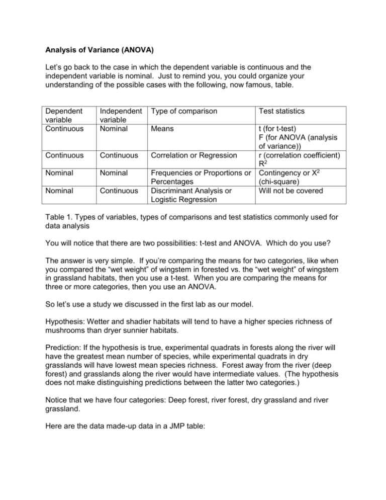
Analysis of Variance (ANOVA)
Let’s go back to the case in which the dependent variable is continuous and the
independent variable is nominal. Just to remind you, you could organize your
understanding of the possible cases with the following, now famous, table.
Dependent
variable
Continuous
Independent
variable
Nominal
Type of comparison
Test statistics
Means
Continuous
Continuous
Correlation or Regression
Nominal
Nominal
Nominal
Continuous
Frequencies or Proportions or
Percentages
Discriminant Analysis or
Logistic Regression
t (for t-test)
F (for ANOVA (analysis
of variance))
r (correlation coefficient)
R2
Contingency or X2
(chi-square)
Will not be covered
Table 1. Types of variables, types of comparisons and test statistics commonly used for
data analysis
You will notice that there are two possibilities: t-test and ANOVA. Which do you use?
The answer is very simple. If you’re comparing the means for two categories, like when
you compared the “wet weight” of wingstem in forested vs. the “wet weight” of wingstem
in grassland habitats, then you use a t-test. When you are comparing the means for
three or more categories, then you use an ANOVA.
So let’s use a study we discussed in the first lab as our model.
Hypothesis: Wetter and shadier habitats will tend to have a higher species richness of
mushrooms than dryer sunnier habitats.
Prediction: If the hypothesis is true, experimental quadrats in forests along the river will
have the greatest mean number of species, while experimental quadrats in dry
grasslands will have lowest mean species richness. Forest away from the river (deep
forest) and grasslands along the river would have intermediate values. (The hypothesis
does not make distinguishing predictions between the latter two categories.)
Notice that we have four categories: Deep forest, river forest, dry grassland and river
grassland.
Here are the data made-up data in a JMP table:
Table 2. Made-up data of number of different species of mushrooms collected from five
10 X 10 M quadrats in each of four habitats.
Notice that I have a column called “replicate”. Each replicate (or replication) is a sample
of the category. Because we set up five quadrats in each habitat, we have five
replicates for each of the four habitats. I put the replicate numbers in the data table
because it facilitates discussion. For example I could say “replicate 3 of river forest”,
and you would know I’m referring to the quadrat with 12 different species of
mushrooms. Numbering your replicates is very useful for complex data tables.
OK. So we want to test our Prediction that experimental quadrats in river forest will
have the greatest mean number of species, while experimental quadrats in dry
grasslands will have lowest mean species richness. Deep forest and river grasslands
will have intermediate values.
Please do the following:
1. Open or create your data file
2. .Analyze menu  Fit X by Y
3. Select “species richness” as your Y,response, and “habitat” as your X, factor. Click
OK.
4. You will get a graph that shows the data points for each category.
Figure 1. Data points for each of four habitat categories.
5. Then click on the red triangle to the left of “oneway”, drag down to means/anova, and
you should see a new window with a great deal of data on it.
You will also that the graph has been redrawn, with the gray horizontal bar representing
the mean number of species overall, the longer green horizontal bar representing the
mean for each category, and the top and bottom of the diamond shape representing the
95% confidence intervals. Based on these samples we are 95% confident that the true
mean for that category falls between the top tip and bottom tip of the diamond.
We won’t worry about the meaning of the two shorter green horizontal bars for now.
Here are the essential data from this table:
A. In the “Summary of Fit” table, the overall mean of response = 3.8. You won’t report
that, but it’s nice to know.
B. In the Analysis of Variance (ANOVA) table, you will note the DF (degrees of freedom)
for habitat = 3, and DF for error = 16. The F-ratio is 11.90, and P = 0.0002. You would
report that as follows: “F3,16 = 11.90, P = 0.0002.”
So what does this mean? Because the P-value is so low (much less than 0.05), we can
support our hypothesis that species richness is significantly different for different
habitats.
C. In the “Means for Oneway Anova” table, you will see the means and standard errors
reported for each category. Beware! Those standard errors are for the entire
sample, not for the individual categories. To get the standard error for each
category, click on the red triangle and drag to “Means and Std Dev.” You’ll get the
following:
These are the correct values for means, standard deviations, and standard errors. Your
report should include (either in the text of the paper, in a figure, or in a table) the means
for each category, and either the standard error of the mean, or the standard deviation.
The frustrating thing is that while we now know that habitat influences mushroom
species richness, we still don’t know which category is significantly different from which.
In other words we still haven’t fully tested the predictions of our hypothesis.
There’s only one more step.
6. Go back to that little red triangle, drag to “compare means”, then drag to all “pairs
Tukey HSD”. You will get the box below:
The bottom portion of this output is of relevance. You will notice that “Levels not
connected by same letter are significantly different.” (for our purpose levels =
categories). For example the mean (7.6) for River forest has an A next to it. Thus its
mean is significantly greater than the 2 categories that don’t have an A next to them
(both grassland categories), but it isn’t significantly greater than Deep forest (which also
has an A next to it). Similarly Deep forest’s mean is significantly greater than Dry
grassland’s mean, but not River grassland (Because Deep forest and River grassland
both share the letter B).
So that’s how we will be comparing means in this class when there are more than two
categories for a nominal independent variable.
Notice that I used the term significantly greater rather than significantly different - if the
means are different I want to know which is greater than which.
Have we supported, or failed to support our research hypothesis?