EPSRC Summer School 2007, Ian Drumm, FDTD
Dr Ian Drumm, The University of Salford
The Finite Difference Time Domain method (FDTD) uses centre-difference representations of the continuous partial differential equations to create iterative numerical models of wave propagation.
Initially developed for electromagnetic problems [1] the technique has potential application in acoustic prediction [2] [3].
In this tutorial you will learn how to implement a simple 1D FDTD using matlab.
The acoustic application of the technique considers wave propagation in a medium using the equations for change of acoustic particle velocity w
and pressure p with respect to time.

 
1
 (1)

   w (2) where

is the medium density and K is the medium bulk modulus.
Gradient operator

 f
, x


, y




Divergence operator f
 x

 y


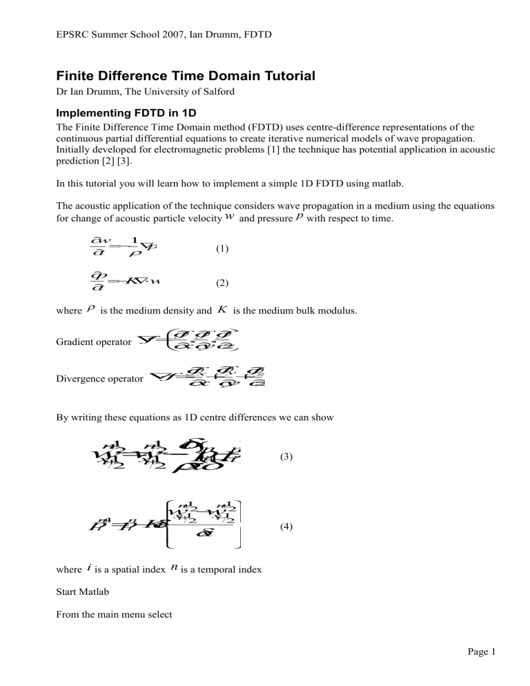
By writing these equations as 1D centre differences we can show
1 w
1
2
1
2

 
(3) p 1
 n i


 x
1
2
1
2
 x x
1
2
1
2



(4) where i is a spatial index n
Start Matlab
From the main menu select is a temporal index
Page 1

EPSRC Summer School 2007, Ian Drumm, FDTD
File->New->M-File
Hence in the edit window type close all; clear all;
Then save the file to D:\ with the file name ‘myFDTD’. This is a matlab source file where you will implement your FDTD model.
We need to create arrays for pressure and velocity with a spatial width of say 100 points and temporal width of 2 for current and previous values. spatialWidth=100; temporalWidth=2; p=zeros(spatialWidth,temporalWidth); v=zeros(spatialWidth,temporalWidth);
If our model is to represent a waveguide of a given length (say 2m) we can evaluate the spatial resolution with length=2; dx=length/spatialWidth;
Hence we can determine the temporal resolution using the courant limit s


 t c

1
N
which is 1 for
1D case. Hence type c=340; dt=dx/c;
We also need to set density and modulus rho=1.21; k=rho*c^2;
Page 2

EPSRC Summer School 2007, Ian Drumm, FDTD
Let’s say we want to run the simulation for five seconds then we will need declare and set ‘duration’ and ‘iterations’ variables with duration=5; iterations=duration/dt;
Let’s decide on an excitation point half way along the waveguide with excitationPoint=spatialWidth/2;
Hence given the necessary parameters we can construct a loop that iterates across the waveguide to set pressures and velocities. This loop is then nested within another loop that iterates for successive time steps. Add to your matlab source code the following… for n=2:iterations
t=n*dt;
for i=2: spatialWidth-1
p(i,1)=p(i,2)-k*dt/dx*(v(i+1,2)-v(i,2));
if i==excitationPoint
p(i,1)=cos(2*pi*500*t);
end
v(i,1)=v(i,2)-(1/rho)*dt/dx*(p(i,1)-p(i-1,1));
p(i,2)=p(i,1);
v(i,2)=v(i,1);
end
plot(p(:,2))
axis([0 spatialWidth -2 2]);
frame = getframe(); end
The loop generates a sine wave at the excitation point which in propagated in both directions along the waveguide as shown in figure 1.
Page 3

EPSRC Summer School 2007, Ian Drumm, FDTD
Figure 1
Note when the wave reaches the end of the ends of the waveguide it is reflected back into the medium.
This is a problem for most simulations that can be solved with the implementation of perfectly match layers (PMLs) – see later.
If FDTD is to be used for analysis of a system across a range of frequencies an alternative source function is needed. For example a Gaussian pulse f
 e
 t
0
) /

)
2 gives an impulse like source with a range of frequency content determined by the pulse width

. The smaller the pulse width the higher the frequency range though clearly the discrete model has a frequency range limited by its resolution which if exceed will generate unacceptable numerical errors.
Figure 2 shows a Gaussian pulse where
 
1 , t
0

5
.
Figure 2
Page 4

EPSRC Summer School 2007, Ian Drumm, FDTD
Edit the matlab source to comment out the old source function for a new one. Bold text indicates changes to matlab code. close all; clear all; spatialWidth=100; temporalWidth=2; p=zeros(spatialWidth+1,temporalWidth); v=zeros(spatialWidth+1,temporalWidth); length=2; dx=length/spatialWidth; c=340; dt=dx/c; rho=1.21;
K=rho*c^2 duration=5; iterations=duration/dt; excitationPoint=spatialWidth/2; for n=2:iterations
t=n*dt;
for i=2: spatialWidth-1
p(i,1)=p(i,2)-K*dt/dx*(v(i+1,2)-v(i,2));
if i==excitationPoint
%p(i,1)=cos(2*pi*500*t);
sigma=0.0005;
t0=3*sigma;
fs=exp( - ((t-t0)/0.0005)^2 );
p(i,1)=fs;
end
v(i,1)=v(i,2)-(1/rho)*dt/dx*(p(i,1)-p(i-1,1));
p(i,2)=p(i,1);
v(i,2)=v(i,1);
end
plot(p(:,2))
axis([0 spatialWidth -2 2]);
frame = getframe(); end
The code generates a Gaussian pulse as a hard source. Notice how waves reflected from the left and right boundaries interfere with it.
You could instead implement a soft source with p(i,1)=p(i,1)+fs;
This doesn’t scatter incident waves however notice how the source function appears to have changed.
This is because when you add pressure at a point the resultant pressure is the sum of the medium’s behaviour and the pressure of your source function.
You could compensate for the medium’s response by implementing a transparent source with
Page 5

EPSRC Summer School 2007, Ian Drumm, FDTD
p(i,1)=p(i,1)+fs+fsPrev;
fsPrev=fs; where fsPrev=0 is declared at the top of the code. This is fine for the 1D scenario however for 2D and
3D the problem is somewhat harder requiring you to add the convolution of the medium’s impulse response and the source history [4].
Page 6

EPSRC Summer School 2007, Ian Drumm, FDTD
When a wave reaches the ends of the waveguide it is reflected back into the medium. This is a problem for most simulations that can be solved with the implementation of perfectly match layers
(PMLs). Originally developed by Berenger [5], the technique specifies a new region that surrounds the
FDTD domain where a set of non physical equations are applied giving a high attenuation. For our 1D case the equations are
 1
(5)



 
K w
Where

is the attenuation coefficient.
Equations (5) and (6) give the solution w x
  p
 z


(6)



 xw c

(8)
Clearly by setting attenuation factor
 
0 we get back to the original FDTD equations (1) and (2) hence it can be shown that the wave speed is the same for medium and PML region as is the impedance p
(9)
Berenger hence showed that the PML boundary is theoretically reflection less, though in practice one has to give the PML boundary a width of say 10 elements and gradually introduce the absorption.
To implement in 1D our update equation (5) for the PML can be given using exponential differencing


  
  x n  n p (9)

(10) similarly (6) becomes
 i p i e

 t




1
2
1 
1

1


(11)
Page 7

EPSRC Summer School 2007, Ian Drumm, FDTD
1 p i
 t e

 
 

2 
1 w


(12)
For our implementation we’ll create a PML region of 10 elements and hence gradually introduce the absorption such that
 i
 


2
PML
(13)
Where the maximum absorption for 1/10 of the PML will be e
  
0 .
1
 1
 ln(
(14) where x i
is the distance moved into PML and x
PML
is PML width.
Edit the previous matlab file to include a PML to the right hand side of the simulation. Key changes are in bold. close all; clear all; spatialWidth=100; temporalWidth=2; p=zeros(spatialWidth+1,temporalWidth); v=zeros(spatialWidth+1,temporalWidth); length=2; dx=length/spatialWidth; c=340; dt=dx/c; rho=1.21;
K=rho*c^2 duration=5; iterations=duration/dt; excitationPoint=spatialWidth/2; xPML=10; for n=2:iterations
t=n*dt;
for i=2: spatialWidth-1
if i>(spatialWidth-xPML)
xi=xPML-(spatialWidth-i);
a0=log(10)/(K*dt);
a1=a0*(xi/xPML)^2;
a2=a0*((xi-1/2)/xPML)^2;
p(i,1)=exp(-(a1*K)*dt)*p(i,2)-(1-exp(-(a1*K)*dt))/(a1*K)*K*1/dx*(v(i+1,2)-v(i,2));
v(i,1)=exp(-(a2*K)*dt)*v(i,2)-(1-exp(-(a2*K)*dt))/(a2*K)*(1/rho)*1/dx*(p(i,1)-p(i-1,1));
Page 8

EPSRC Summer School 2007, Ian Drumm, FDTD
else
p(i,1)=p(i,2)-K*dt/dx*(v(i+1,2)-v(i,2));
if i==excitationPoint
%p(i,1)=cos(2*pi*500*t);
sigma=0.0005;
t0=3*sigma;
fs=exp( - ((t-t0)/0.0005)^2 );
p(i,1)=p(i,1)+fs;
end
v(i,1)=v(i,2)-(1/rho)*dt/dx*(p(i,1)-p(i-1,1)); end
p(i,2)=p(i,1);
v(i,2)=v(i,1);
end
plot(p(:,2))
axis([0 spatialWidth -2 2]);
frame = getframe(); end
Note two absorption coefficients a1 and a2 are created to take account of pressure and velocity being
½ and element apart in the staggered grid.
Can you implement a PML for the left hand side as well?
What is the effect of changing the courant number s
to values greater than or less than one?
How might you emulate a reflecting surface in the model?
What are the update equations for 2D and 3D scenarios?
1) K. S. Yee, “Numerical solution of initial boundary value problems involving Maxwell’s equations in isotropic media,” IEEE Trans. Antennas Propagat.
14 , 302–307 (1966).
2) J.G. Meloney and K.E. Cummings, “Adaption of FDTD techniques to acoustic modelling”,11 th
Annu. Rev. Prog. Applied Computational Electromagnetics, Vol.2, 724 (1995)
3) D. Botteldooren. “Finite-difference time-domain simulation of low frequency room acoustic problems.”, J. Acoust. Soc. Am., 98(6):3302-- 3308, 1995.
4) J.B. Schneider, C.L. Wagner, S.L. Broschat, “Implementation of transparent sources embedded in acoustic finite difference time domain grids”, J. Acoust. Soc. Am Vol 133, No. 1, 136-142, January
1998.
5) J.P. Berenger, “A perfectly matched layer for the absorption of electromagnetic waves’. J.
Computational Physics, vol 114, 185-200, 1994.
Page 9

EPSRC Summer School 2007, Ian Drumm, FDTD
6) X. Yuan, D.Borrup, M.Berggeren, J. Wiskin, S. Johnson, “Simulation of acoustics wave propagation in dispersive media with relaxation loses by using FDTD method with PML absorbing boundary condition” IEE Trans Ultrason 1996.
Page 10