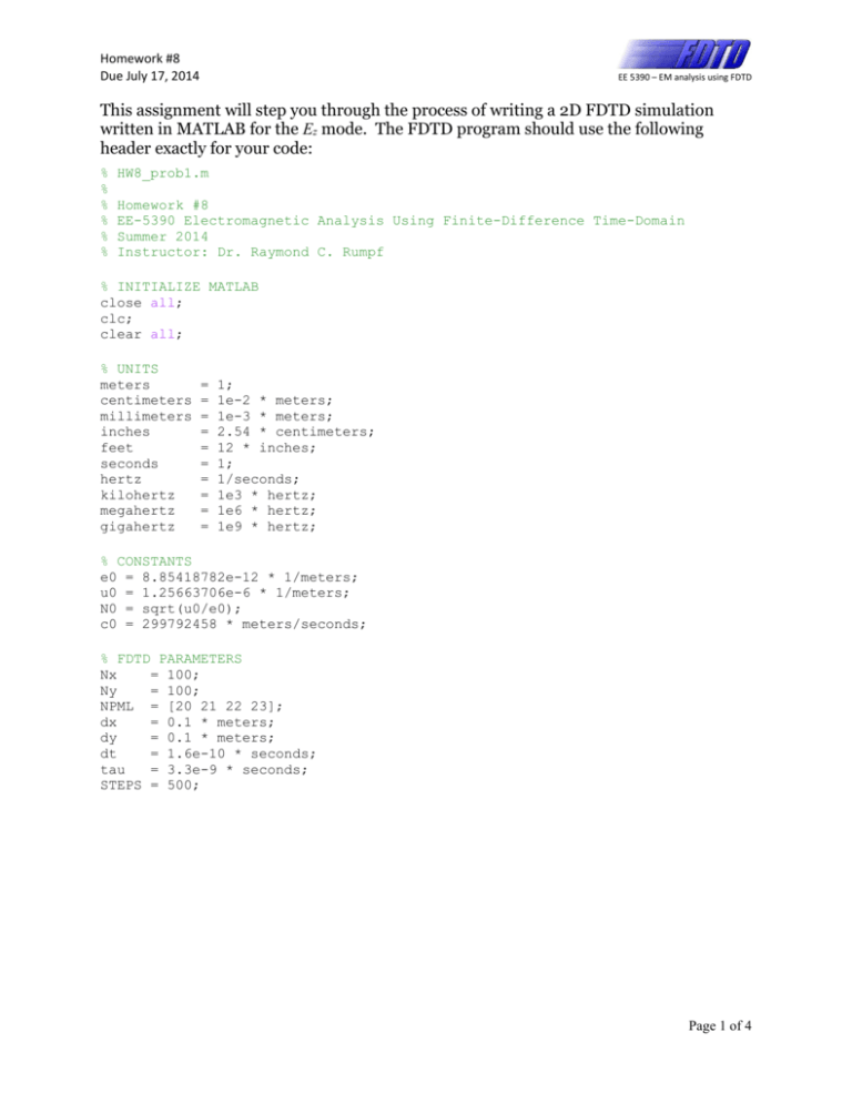
Homework #8
Due July 17, 2014
EE 5390 – EM analysis using FDTD
This assignment will step you through the process of writing a 2D FDTD simulation
written in MATLAB for the Ez mode. The FDTD program should use the following
header exactly for your code:
%
%
%
%
%
%
HW8_prob1.m
Homework #8
EE-5390 Electromagnetic Analysis Using Finite-Difference Time-Domain
Summer 2014
Instructor: Dr. Raymond C. Rumpf
% INITIALIZE MATLAB
close all;
clc;
clear all;
% UNITS
meters
centimeters
millimeters
inches
feet
seconds
hertz
kilohertz
megahertz
gigahertz
=
=
=
=
=
=
=
=
=
=
1;
1e-2 * meters;
1e-3 * meters;
2.54 * centimeters;
12 * inches;
1;
1/seconds;
1e3 * hertz;
1e6 * hertz;
1e9 * hertz;
% CONSTANTS
e0 = 8.85418782e-12 * 1/meters;
u0 = 1.25663706e-6 * 1/meters;
N0 = sqrt(u0/e0);
c0 = 299792458 * meters/seconds;
% FDTD PARAMETERS
Nx
= 100;
Ny
= 100;
NPML = [20 21 22 23];
dx
= 0.1 * meters;
dy
= 0.1 * meters;
dt
= 1.6e-10 * seconds;
tau
= 3.3e-9 * seconds;
STEPS = 500;
Page 1 of 4
Homework #8
Due July 17, 2014
EE 5390 – EM analysis using FDTD
Problem #1: Calculate the PML Parameters
For Problem #1, add to the header above to calculate the PML parameters sigx and
sigy on a 2× grid. That is, create two 2D arrays in memory (sigx and sigy) and
assign values to each point according to Lecture 15. The size of the PML at each
boundary is defined by the 1×4 array NPML. The first number corresponds to the x=0
boundary (x-low), the second is the x=Nx boundary (x -high), the third is the y=0
boundary (y-low), and the fourth is the y=Ny boundary (y-high).
To test your code, the final statement in your program should be
% TEST CONDUCTIVITY TERMS
test_hw8_prob1
If your code creates sigx and sigy correctly, you should receive the message
“Problem #1 items appear to be correct!!” at the command prompt after
running your code.
Problem #2: Calculate the Update Coefficients for the Ez Mode
Add to your code developed for Problem #1 to calculate the update coefficients for the Ez
mode. First, you will need to define your materials arrays URxx, URyy, and ERzz. Set
all of these to free space (i.e. 1.0). Second, add the code to calculate the following update
coefficients:
mHx1, mHx2, mHx3
mHy1, mHy2, mHy3
mDz1, mDz2, mDz4
mEz1
To test your code, the final statement in this program should be
% TEST VALUES
test_hw8_prob2
If your code is working correctly, you should receive the following message in the
command window after running your code.
Problem #1 items appear to be correct!!
Problem #2 items appear to be correct!!
>>
Page 2 of 4
Homework #8
Due July 17, 2014
EE 5390 – EM analysis using FDTD
Problem #3: Implement the 2D FDTD Algorithm for the Ez Mode
Modify your code from Problem #2 by adding the following functions:






Calculate a simple Gaussian source (not TF/SF…yet) just like you did for 1DFDTD.
Initialize the fields to zero: Hx=Hy=Dz=Ez=0
Initialize the curl terms to zero: CEx=DEy=CHZ=0
Initialize the integration terms to zero: ICEx=ICEy=IDz=0
Add the main FDTD loop following the block diagram in Lecture 15 exactly.
Add a segment of code inside the main FDTD loop to visualize the Ez field. Use
the draw2d() function provided on the course website. This function
superimposes the electric field onto the permittivity.
If your code is calculating the update coefficients correctly, you should get the following
result at T = 200. Please provide your field visualization at T = 200. Make your final
plot look professional and “publication ready.”
Page 3 of 4
Homework #8
Due July 17, 2014
EE 5390 – EM analysis using FDTD
Here is the help information for the draw2d() function:
draw2d
Draw Field Superimposed on Materials for 2D FDTD
h = draw2d(xa,ya,ER,E,NPML)
h = draw2d(xa,ya,ER,E,NPML,OPTS)
This MATLAB function superimposes the field on top of the materials
and plots the image to the current axes. Fruther, it highlights the
PML regions.
INPUT ARGUMENTS
================
xa, ya
Axis vectors
ER
Permittivity
E
The electric
NPML
[xlo xhi ylo
OPTS
.emax
.cmap
.NCOL
listing the position of each cell in the grid
function across the 2D grid
field across the 2D grid
yhi] size of the PML
Options (Optional)
maximum value of the electric field
custom colormap
USA, Mexico, or any MATLAB colormap
could also be a Nx3 array for custom colormap
number of shades of color (default 64)
OUTPUT ARGUMENTS
================
h
Handle to the plot
Page 4 of 4