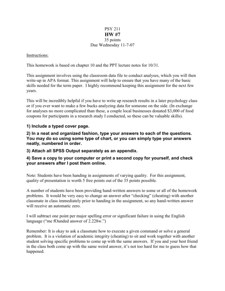
PSY 211
HW #7
35 points
Due Wednesday 11-7-07
Instructions:
This homework is based on chapter 10 and the PPT lecture notes for 10/31.
This assignment involves using the classroom data file to conduct analyses, which you will then
write-up in APA format. This assignment will help to ensure that you have many of the basic
skills needed for the term paper. I highly recommend keeping this assignment for the next few
years.
This will be incredibly helpful if you have to write up research results in a later psychology class
or if you ever want to make a few bucks analyzing data for someone on the side. (In exchange
for analyses no more complicated than these, a couple local businesses donated $3,000 of food
coupons for participants in a research study I conducted, so these can be valuable skills).
1) Include a typed cover page.
2) In a neat and organized fashion, type your answers to each of the questions.
You may do so using some type of chart, or you can simply type your answers
neatly, numbered in order.
3) Attach all SPSS Output separately as an appendix.
4) Save a copy to your computer or print a second copy for yourself, and check
your answers after I post them online.
Note: Students have been handing in assignments of varying quality. For this assignment,
quality of presentation is worth 5 free points out of the 35 points possible.
A number of students have been providing hand-written answers to some or all of the homework
problems. It would be very easy to change an answer after “checking” (cheating) with another
classmate in class immediately prior to handing in the assignment, so any hand-written answer
will receive an automatic zero.
I will subtract one point per major spelling error or significant failure in using the English
language (“me fOunded answer of 2.228w.”)
Remember: It is okay to ask a classmate how to execute a given command or solve a general
problem. It is a violation of academic integrity (cheating) to sit and work together with another
student solving specific problems to come up with the same answers. If you and your best friend
in the class both come up with the same weird answer, it’s not too hard for me to guess how that
happened.
APA-format of Write-ups
Here are some examples of how to write results in APA-style. This is just a guide. If you are a
good writer, it is okay to deviate from this somewhat. Remember, p-values can be recorded
exactly (e.g. p = .013, p = .46, etc.) or by merely stating significance (p < .05), or by merely
stating non-significance (ns). It is okay to separate statistical results from the rest of the sentence
by enclosing statistics in parentheses or by using commas. For correlations, provide the r value
and p value. For regression, provide the initial correlational results, then conduct the regression,
and provide the R2 and p-value. For t-tests, provide the Cohen’s d (calculated by hand, do not
need to show hand-calculations this time), t-value, and p-value.
Correlation (Statistically Significant):
The correlation between IQ and hours of television watched was significant, r = -.35, p = .02.
That is, people who were smarter watched moderately less television.
The correlation between IQ and hours of television watched was significant, r = -.35, p < .05.
That is, people who were smarter watched moderately less television.
For correlations of magnitude < .10, we say something to the effect of “no sizeable relationship.”
For correlations of magnitude .10 to .29, say the relationship is “small” or use a related synonym.
For correlations of magnitude .30 to .49, say the relationship is “medium” or “modest” or some
other synonym. For correlations of .50 or greater, say “large” or some other synonym.
Correlation (Non-Significant):
IQ and number of hours of television watched were not significantly related, r = .08, p = .67.
Thus, one’s level of intelligence was not related to time spent watching television.
IQ and number of hours of television watched were not sizably related, r = .08, ns. Thus, one’s
level of intelligence was not related to time spent watching TV.
Multiple Regression (after discussion of correlational results):
Family stress (r = .48, p < .05), work stress (r = .56, p < .05), and school stress (r = .21, p < .05)
all significantly predicted overall life stress. However, social support did not predict level of life
stress, r = .03, ns. Thus, although social support was not related to life stress, one’s level of
school stress was slightly related, family stress was modestly related, and work stress was
strongly related to level of life stress. To examine the overall contribution of the three
significant predictors (school stress, family stress, and life stress) in accounting for life stress,
multiple regression was used. The results of the multiple regression analysis indicate that these
three predictors accounted for a large proportion of the variance in life stress, R2 = .40, p < .05.
Thus, school stress, family stress, and work stress together account for 40% of the differences in
overall life stress.
t-tests (Statistically Significant)
Males (M = 2.0, SD = 0.6) differed from females (M = 5.0, SD = 0.4) in terms of number of pairs
of shoes owned. This difference was large and statistically significant, d = 6.0, t(128) = 3.89, p <
.05. In conclusion, males tend to own fewer pairs of shoes than females.
Cohen’s d is a measure of how big the relationship is (effect size), see 10/31 PPT notes for
details. d = (M1 – M2) / s where M1 is the mean of the first group (2.0), and M2 is the mean of
the second group (5.0), and s is the average standard deviation across groups [(.6+.4)/2 = .5].
d = (2-5)/.5 = -3/.5 = -6. You can make d positive if you like , just make sure you interpret it
correctly (males are lower than females). When d has a magnitude less than .2, we say
something like “there was no relationship;” .2-.49 means “a small relationship;” .5-.79 means “a
modest relationship;” .8 or higher means “a large relationship.” There is no maximum value for
d.
The values in the parentheses after the t is the degrees of freedom for the whole sample, which is
provided by SPSS, but also equals the total sample size minus 2, that is N-2.
dftotal = df1 + df2 = (n1 – 1) + (n2 – 1) = N -2
t-tests (non-Significant)
Males (M = 2.9, SD = 0.6) did not differ from females (M = 3.1, SD = 0.4) in terms of number of
pairs of shoes owned. This difference was small and not statistically significant, d = 0.4, t(128)
= 1.12, ns. In conclusion, males tend to own about as many pairs of shoes as females.
HW #7
Review: Correlation and Regression
1) In APA style, write up the results for analyses examining the three correlations between these
variables: Self-reported intelligence (#55), Attractiveness (#66), and Life Satisfaction (#78).
2) In APA style, write up the results for a multiple regression analysis. First, examine how well
three predictors [Self-reported intelligence (#55), Attractiveness (#66), and Life Satisfaction
(#78)] correlate with an outcome [Overwhelm (#75)]. Then, conduct a multiple regression
analysis, using only the two predictors that significantly predict Overwhelm (ignoring the one
bad predictor).
Note on finding the multiple regression value you need for the write-up: R2 is in the second box
of the regression Output (3rd column over, “R Square”). The p-value we need is in the third box
of the Output (right-most column, “Sig.”).
t-tests – Easy
Between-group t-tests can be easily conducted in SPSS. Go to the Analyze menu, point to
“Compare Means”, and choose “Independent-Samples T Test…” from the menu. A pop-up box
will appear. We always put the independent variable (category or group status) in the “Grouping
Variable” section of the box, and the dependent variable (continuous variable or outcome
variable) in the “Test Variable(s):” box. SPSS lets us put multiple variables in the “Test
Variable(s):” box if we want to examine how group status impacts multiple outcome variables.
Put Gender (#2) in the “Grouping Variable” section of the box, and put both Beauty Concerns
(#44) and War Support (#70) in the “Test Variable(s):” box. At this point, you will notice that
the OK button is still in gray. We must do one final step before it will run the analyses. After
moving Gender to the “Grouping Variables” section, click on it once to select it. Then click on
the Define Groups… box. This makes another pop-up box appear. Where is says “Group 1:”
type in “0” because females were coded as “0” and for “Group 2:” type in “1” because males
were coded as a “1”. Click Continue. Click OK. The Output should appear.
3) Report the results in APA format (you will need to calculate Cohen’s d by hand, but it’s easy).
See the lecture notes for where to find relevant information in the Output.
t-tests – Moderate Difficulty
One weakness of the t-test is that is can only be used to compared results across groups that only
have two categories. The above example works fine for categorical variables that only have two
categories (#1 - #20), but some of our categorical variables have more than two categories (#21 #31). Later in the course, we will learn to analyze these variables using ANOVA. For now,
however, we can stick to just analyzing two of the categories from our multi-category variables.
One of the variables that has multiple categories is Favorite Color (#28). The categories are
below:
1 = Red, 2 = Green, 3 = Blue, 4 = Yellow, 5 = Pink, 6 = Black, 7 = Orange, 8 = Purple, 9 = Other
We might want to examine whether someone’s favorite color is related to their level of
Depression (#46). We cannot correlate favorite color with level of depression, because color is
not a continuous variable (the numbers assigned to the colors are arbitrary not meaningful). If
we knew ANOVA, we could look at level of depression for each of these colors and compare all
categories at the same time. Because t-tests only let us compare two categories, let use compare
people who said their favorite colors was Blue to those who said Red.
4) Run a t-test comparing favorite color to depression. Go through the same t-test steps as
before, but the trick is that in the Define Groups… pop-up from the t-test window, you just need
to specify which categories to look at. Choose “1” and “3” because Red = 1 and Blue = 3 (this is
similar to the previous problem, where we specified females = 0 and males = 1). Then, run a
second t-test where you compare Blue to some other favorite color, also examining level of
depression. Report both results in APA-style, and remember to calculate Cohen’s d.
t-test – Complex
The previous problem shows one way of handling these multi-category variables using t-tests.
Another way would be to change how the variables are coded. For example, you could group all
of the favorite colors into two categories: Red and non-Red, rather than just examining Red vs.
Blue. You could also put Black and Blue in one category and all other colors in a different
category. We’ll practice using the religion variable.
Go to the Transform menu. Point to “Recode” and choose “Into Different Variables…” from the
menu, making a pop-up appear. This is where we go to recode one variable into a different
variable with fewer categories. Move Religion (#23) into the section of the box labeled
“Numeric Variable -> Output Variable.” In the section of the window on the right side, type a
variable name for the new, two-category variable we are generating by typing something like
“religion2” in the “Name:” section. You can also type a label for the variable, which will appear
in the Output, by typing something in the “Label:” section (I chose “religion2” again for good
measure). Click on the Change button. This tells SPSS, that we are recoding the Religion
variable into a variable called religion2, which will have different categories. You will notice
that the OK button is still gray because we need to specify how the variable will be recoded.
Click on the Old and New Values… button. Initially, the religion variable had the following
categories: 0 = Non-religious, 1 = Christianity, 2 = Agnosticism, 3 = Atheism, 4 = Other. We
want to reorganize the data into just two categories. We could do this any number of ways, but
for this we will compare Christians (1) to non-Christians (all others: 0, 2, 3, 4). In the window
that popped up, type in a “1” in the “Value:” area of the “Old Value” section and a “1” in the
“Value:” section of the “New Value” section; then click the Add button. This says that anyone
who previously had a numeric value of “1” will still have a value of “1”. Now type a “0” for Old
Value and a “2” for New Value and click Add. Now type a “2” for Old Value and a “2” for New
Value and click Add. Now type a “3” for Old Value and a “2” for New Value and click Add.
Now type a “4” for Old Value and a “2” for New Value and click Add. This says that anyone
who previously had a value of 0, 2, 3, or 4 will now be coded as a 2. Click the Continue button.
Click the OK button. [There are more efficient ways to use this pop-up window, so feel free to
go back and experiment when you are done.]
Go back to your “Data View” window. If you scroll all the way to the last variable on the right,
you should see your new variable, “religion2”. Scroll up and down to make sure participants
only have a value of “1” or “2”. Otherwise, you messed up!
Now, you can do a t-test on the religion2 variable (see the “t-test Basics” section above). Do a ttest examining how religion (Christianity vs. non-Christianity) compares to Extraversion (#56).
Remember to choose the appropriate numbers to specify each category in the Define Groups…
pop-up window, where Christianity = 1, and all others = 2.
5) Report the results of this t-test in APA-format, and remember to include Cohen’s d.
6). Recode the Hero variable (#22). Previously, the variable was coded like this:
1 = Mom, 2 = Dad, 3 = Sibling, 4 = Other relative, 5 = Friend, 6 = Romantic Partner, 7 = Famous
person, 8 = Teacher/Coach, 9 = Other
Recode the variable so that parents (1 and 2) are grouped into one category and all others (3-9)
are coded as a different category. Run a t-test comparing this two-category (dichotomous) hero
variable to Healthy Habits (#74). Write-up the result in APA-format, including Cohen’s d.
Answers
These are just examples of high-quality responses. There are multiple correct answers for each
problem.
1. The results of the correlational analyses indicated that attractiveness was slightly correlated
with self-reported intelligence (r = .21, p < .001) and slightly correlated with life satisfaction (r =
.19, p = .001). However, self-reported intelligence and life satisfaction were not correlated (r =
.09, ns). Thus, attractive people tended to report being more intelligent and having more
satisfying lives, but life satisfaction and intelligence were not related.
2. Level of overwhelm was slightly correlated with self-reported intelligence (r = -.13, p = .02)
and modestly correlated with life satisfaction (r = -.30, p < .001). However, level of overwhelm
was not related to attractiveness (r = -.03, ns). Thus, people who were overwhelmed reported
slightly lower levels of intelligence and modestly lower levels of life satisfaction. Multiple
regression was used to determine the overall contribution of intelligence and life satisfaction in
predicting overwhelm. The two predictors combined to explain 10% of the variance in level of
overwhelm, R2 = .10, p < .001, which was a modest effect.
3. Females (M = 4.46, SD = 1.46) tended to report greater beauty concerns than males (M = 3.99,
SD = 1.52). This effect was small, d = .32, and statistically significant, t(324) = 2.68, p = .008.
Additionally, females (M = 3.06, SD = 1.84) tended to report about the same level of war support
as males (M = 3.18, SD = 1.87), and this difference was not statistically significant, d = .12,
t(324) = 0.53, ns. Thus, males and females tended to have similar levels of war support, but
females had greater beauty concerns than males.
[Note: It is difficult to determine why anyone would simultaneously look at gender differences
on these very unrelated variables, war support and beauty concerns. Hopefully the focus of your
term paper is a bit more sensible.]
4. Commonly, depression is characterized as having the blues. T-tests were used to determine if
favorite color was related to depression. People who said their favorite color was red (M = 1.45,
SD = 1.55) actually had higher levels of depression than people who reported having a favorite
color of blue (M = 1.13, SD = 1.30). This effect was small, d = 0.23, and due to low sample size
in the red group was not statistically significant, t(134) = 1.15, ns. Interestingly, however,
people who chose a favorite color of black (M = 2.29, SD = 1.82) had higher levels of depression
than those who chose blue (M = 1.13, SD = 1.30). This effect was modest, d = 0.74, and
statistically significant, t(117) = 2.96, p = .004. Thus, having a favorite color of blue is not
related to depression; in fact, having a favorite color of black is more related to depressive
symptoms.
[Note: In the second comparison, it was your choice which color to compare to blue, so the
second part of this write-up will vary from person to person.]
5. A t-test was used to examine whether religious worldview was related to the trait of
extraversion. People who reported being Christian (M = 4.49, SD = 1.41) had about the same
level of extraversion as those who described themselves as having a different worldview (M =
4.65, SD = 1.48). This effect was not significant, d = 0.10, t(324) = 0.90, ns, indicating that
worldview was not related to extraversion.
6. A t-test was used to determine if one’s self-reported hero was related to health habits. People
who indicated that one of their parents was their hero (M = 4.91, SD = 1.48) tended to have a
lower level of health habits than those listing someone else as a hero (M = 5.35, SD = 1.59).
This effect was small, d = 0.29, and statistically significant, t(324) = 2.60, p = .01, indicating that
having a non-parent as a hero was related to better health behavior.
[I cannot think of a good reason why this result would occur, but it seems interesting.]
Appendix
Correlations
66. Attractivenes s
55. Self-reported
Intelligence
78. Life Satisfaction
Pearson Correlation
Sig. (2-tailed)
N
Pearson Correlation
Sig. (2-tailed)
N
Pearson Correlation
Sig. (2-tailed)
N
55.
Self-reported
78. Life
Intelligence
Satisfaction
.211**
.191**
.000
.001
326
326
326
.211**
1
.086
.000
.122
326
326
326
.191**
.086
1
.001
.122
326
326
326
66.
Attractiveness
1
**. Correlation is significant at the 0.01 level (2-tailed).
Correlations
66. Attractivenes s
55. Self-reported
Intelligence
78. Life Satisfaction
75. Overwhelmed
Pearson Correlation
Sig. (2-tailed)
N
Pearson Correlation
Sig. (2-tailed)
N
Pearson Correlation
Sig. (2-tailed)
N
Pearson Correlation
Sig. (2-tailed)
N
55.
Self-reported
78. Life
75.
Intelligence
Satisfaction
Overwhelmed
.211**
.191**
-.036
.000
.001
.523
326
326
326
326
.211**
1
.086
-.133*
.000
.122
.016
326
326
326
326
.191**
.086
1
-.295**
.001
.122
.000
326
326
326
326
-.036
-.133*
-.295**
1
.523
.016
.000
326
326
326
326
66.
Attractiveness
1
**. Correlation is significant at the 0.01 level (2-tailed).
*. Correlation is significant at the 0.05 level (2-tailed).
Variables Entered/Removedb
Model
1
Variables
Entered
78. Life
Satisfactio
n, 55.
Self-report
ed
Intelligenc
a
e
Variables
Removed
Method
.
Enter
a. All requested variables entered.
b. Dependent Variable: 75. Overwhelmed
Model Summary
Model
1
R
.314a
R Square
.099
Adjusted
R Square
.093
Std. Error of
the Estimate
1.5667
a. Predictors: (Constant), 78. Life Satisfaction, 55.
Self-reported Intelligence
ANOVAb
Model
1
Regres sion
Residual
Total
Sum of
Squares
86.966
792.838
879.804
df
2
323
325
Mean Square
43.483
2.455
F
17.715
Sig.
.000a
a. Predic tors: (Constant), 78. Life Satis fact ion, 55. Self-reported Intelligence
b. Dependent Variable: 75. Overwhelmed
Coefficientsa
Model
1
(Constant)
55. Self-reported
Intelligence
78. Life Satisfaction
Unstandardized
Coefficients
B
Std. Error
6.708
.537
Standardized
Coefficients
Beta
t
12.495
Sig.
.000
-.170
.083
-.109
-2.047
.041
-.340
.063
-.286
-5.393
.000
a. Dependent Variable: 75. Overwhelmed
Group Sta tisti cs
2. Gender
44. Beauty Concerns Female
Male
70. War Support
Female
Male
N
Mean
4.462
3.990
3.058
3.175
223
103
223
103
St d. Error
Mean
.0978
.1496
.1234
.1838
St d. Deviat ion
1.4603
1.5178
1.8432
1.8652
Independent Samples Test
Levene's Test for
Equality of Variances
F
44. Beauty Concerns
70. War Support
Equal variances
as sumed
Equal variances
not ass umed
Equal variances
as sumed
Equal variances
not ass umed
t-test for Equality of Means
Sig.
.068
t
.794
.142
.707
df
Sig. (2-tailed)
Mean
Difference
Std. Error
Difference
95% Confidence
Interval of the
Difference
Lower
Upper
2.677
324
.008
.4716
.1762
.1250
.8182
2.639
191.759
.009
.4716
.1787
.1191
.8240
-.528
324
.598
-.1165
.2204
-.5501
.3172
-.526
196.410
.599
-.1165
.2214
-.5531
.3201
Group Statistics
46. Depres sion
28. Favorite Color
Red
Blue
N
Mean
1.452
1.133
31
105
Std. Deviation
1.5457
1.3014
Std. Error
Mean
.2776
.1270
Independent Samples Test
Levene's Test for
Equality of Variances
F
46. Depres sion
Equal variances
as sumed
Equal variances
not ass umed
.644
t-test for Equality of Means
Sig.
t
.424
df
Sig. (2-tailed)
Mean
Difference
Std. Error
Difference
1.145
134
.254
.3183
.2780
-.2315
.8681
1.043
43.323
.303
.3183
.3053
-.2973
.9338
Group Statistics
46. Depres sion
28. Favorite Color
Blue
Black
95% Confidence
Interval of the
Difference
Lower
Upper
N
105
14
Mean
1.133
2.286
Std. Deviation
1.3014
1.8157
Std. Error
Mean
.1270
.4853
Independent Samples Test
Levene's Test for
Equality of Variances
F
46. Depres sion
Equal variances
as sumed
Equal variances
not ass umed
t-test for Equality of Means
Sig.
2.650
t
.106
df
Sig. (2-tailed)
Mean
Difference
Std. Error
Difference
95% Confidence
Interval of the
Difference
Lower
Upper
-2.960
117
.004
-1.1524
.3893
-1.9233
-.3815
-2.297
14.833
.037
-1.1524
.5016
-2.2226
-.0822
Group Statistics
56. Extraversion
religion2
1.00
2.00
N
Mean
4.485
4.642
231
95
Std. Error
Mean
.0928
.1518
Std. Deviation
1.4107
1.4798
Independent Samples Test
Levene's Test for
Equality of Variances
F
56. Extraversion
Equal variances
as sumed
Equal variances
not ass umed
t-test for Equality of Means
Sig.
.328
t
.567
df
Sig. (2-tailed)
Mean
Difference
Std. Error
Difference
95% Confidence
Interval of the
Difference
Lower
Upper
-.902
324
.368
-.1573
.1744
-.5004
.1859
-.884
167.815
.378
-.1573
.1779
-.5086
.1940
Group Statistics
74. Healthy Habits
hero2
1.00
2.00
N
179
147
Mean
4.911
5.354
Std. Deviation
1.4813
1.5868
Std. Error
Mean
.1107
.1309
Independent Samples Test
Levene's Test for
Equality of Variances
F
74. Healthy Habits
Equal variances
as sumed
Equal variances
not ass umed
3.321
Sig.
.069
t-test for Equality of Means
t
df
Sig. (2-tailed)
Mean
Difference
Std. Error
Difference
95% Confidence
Interval of the
Difference
Lower
Upper
-2.603
324
.010
-.4431
.1703
-.7781
-.1082
-2.585
302.622
.010
-.4431
.1714
-.7805
-.1058