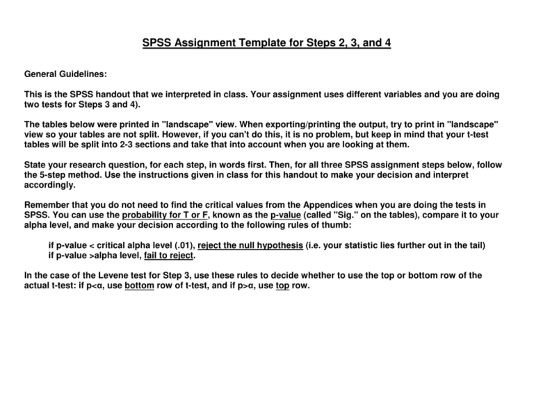
SPSS Assignment Template for Steps 2, 3, and 4
General Guidelines:
This is the SPSS handout that we interpreted in class. Your assignment uses different variables and you are doing
two tests for Steps 3 and 4).
The tables below were printed in "landscape" view. When exporting/printing the output, try to print in "landscape"
view so your tables are not split. However, if you can't do this, it is no problem, but keep in mind that your t-test
tables will be split into 2-3 sections and take that into account when you are looking at them.
State your research question, for each step, in words first. Then, for all three SPSS assignment steps below, follow
the 5-step method. Use the instructions given in class for this handout to make your decision and interpret
accordingly.
Remember that you do not need to find the critical values from the Appendices when you are doing the tests in
SPSS. You can use the probability for T or F, known as the p-value (called "Sig." on the tables), compare it to your
alpha level, and make your decision according to the following rules of thumb:
if p-value < critical alpha level (.01), reject the null hypothesis (i.e. your statistic lies further out in the tail)
if p-value >alpha level, fail to reject.
In the case of the Levene test for Step 3, use these rules to decide whether to use the top or bottom row of the
actual t-test: if p<α, use bottom row of t-test, and if p>α, use top row.
Assignment Step 2: Single-sample T-Test (comparing the sample mean (25.278) to the population or test value of 40
hours)
Research question: Is there a significant difference between the sample mean and the population parameter in # of
hours worked per week?
One-Sample Statistics
N
Number of hours usually
1512
worked at all jobs in a week.
Mean
Std. Deviation
25.278
Std. Error Mean
20.5113
.5275
One-Sample Test
Test Value = 40
t
df
Sig. (2-tailed)
Mean Difference
99% Confidence Interval of the Difference
Lower
Number of hours usually
worked at all jobs in a week.
-27.907
1511
.000
-14.7222
Upper
-16.083
-13.362
Five Step Method:
1. Make Assumptions and meet test requirements. Follow guidelines in powerpoint slides.
2. State the null/alternate hypothesis: H0: µ = 40 (no difference) and H1: µ ≠ 40 (there is a difference)
3. Select the sampling distribution and establish the critical region. Use T-test. (Note that SPSS uses t-test instead of z-test)
Since n>1000, α=.01
4. Compute the test statistic. See One-sample table above for computation.
5. Make a decision:
t = -27.907
p (Sig.) = .000 which is less than α=.01, so reject H0
Interpretation: The sample mean = 25.278 is significantly different from the population mean in # of hours worked per week
(t = -27.907, df=1511, α=.01)
Assignment Step 3: Two-sample T-Test comparing the sample mean for "Yes, limited in activity" (20.680) to the
sample mean for "No, not limited" (27.129) in # of hours worked.
Research question: Is there a significant difference between the sample means in # of hours worked per week?
Group Statistics
Are you limited in the amount
N
Mean
Std. Deviation
Std. Error Mean
or kind of activity you can do
Number of hours usually
Yes
434
20.680
21.2104
1.0182
worked at all jobs in a week.
No
1078
27.129
19.9355
.6072
Independent Samples Test
Levene's Test for Equality of
t-test for Equality of Means
Variances
F
Number of hours usually
Equal variances assumed
20.995
Sig.
t
.000
df
Sig. (2-tailed)
Mean
Std. Error
Difference
Difference
99% Confidence Interval of the Difference
Lower
Upper
-5.586
1510
.000
-6.4494
1.1546
-9.4273
-3.4715
-5.440
757.219
.000
-6.4494
1.1855
-9.5108
-3.3881
worked at all jobs in a
Equal variances not assumed
week.
Five Step Method:
1. Make Assumptions and meet test requirements. Follow guidelines in powerpoint slides for two-sample tests.
2. State the null/alternate hypotheses:
H0: µ1 = µ2 (no difference)
H1: µ1 ≠ µ2 (there is a difference)
3. Select the sampling distribution and establish the critical region. Use T-test. Since n>1000, α=.01 (Note that SPSS uses t-test)
4. Compute the test statistic. See Two-sample table above for computation.
5. Make a decision:
a) Levene's test: Since p (Sig.) = .000 < α=.01, we are going to use the bottom (unequal variances) row of the t-test
b) t = -5.440 p (Sig.) = .000 which is less than α=.01, so reject H0
Interpretation: The sample mean for "Yes" = 20.680 is significantly different* from "No" = 27.167 in # of hours worked per week.
*Report your sig. stats: (t = -5.440, df=757.219, α=.01)
Assignment Step 4: Oneway ANOVA # of Hours Worked by Health Status
Research question: Is there a significant difference in # of hours worked per week by Health Status?
ANOVA
Number of hours usually worked at all jobs in a week.
Sum of Squares
Between Groups
df
Mean Square
13639.472
4
3409.868
Within Groups
621957.012
1506
412.986
Total
635596.484
1510
F
8.257
Sig.
.000
Post Hoc Tests - Homogeneous Subsets
Number of hours usually worked at all jobs in a week.
Tukey B
In general, would you say your
N
Subset for alpha = 0.01
health is:
... poor?
1
2
33
11.869
... fair?
113
18.566
... good?
355
24.594
... excellent?
440
26.192
... very good?
568
27.133
18.566
Five Step Method:
1. Make Assumptions and meet test requirements. Follow guidelines in powerpoint slides for ANOVA.
2. State the null/alternate hypotheses:
H0: µ1= µ2=µ3=µ4=µ5
H1: at least 1 mean is different.
3. Select the sampling distribution and establish the critical region. F-test. Since n>1000, α=.01
4. Compute the test statistic. See ANOVA above for computation, then look at Tukey b table to see which means are different.
5. Make a decision:
a) ANOVA table: F = 8.257, p (Sig.) = .000 < α=.01 therefore reject H0
b) Tukey b test: the mean for poor is significantly different from the means for good, excellent, very good (α=.01)
Interpretation: There is a significant difference in the sample means of # hours worked by health status (F=8.257, df=4,1505, α=.01). The mean for
poor (11.869) is not different from fair (18.566) but is significantly different from good (24.594), excellent (26.192) and very good (27.133).