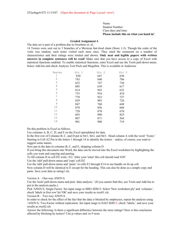
252solngr4-072 11/15/07
(Open this document in 'Page Layout' view!)
Name
Student Number:
Class days and time:
Please include this on what you hand in!
Graded Assignment 4
The data set is part of a problem due to Groebner et. al..
14 Testers were sent out to 3 branches of a Mexican fast-food chain (Store 1-3). Though the order of the
visits was random, each tester visited each store once. They rated the restaurant on a number of
characteristics and their ratings were totaled and shown. Only neat and legible papers with written
answers in complete sentences will be read! Make sure that you have access to a copy of Excel with
statistical functions enabled. To enable statistical functions, enter Excel and use the Tools pull-down menu.
Select Add-Ins and check Analysis Tool Pack and MegaStat. This is available in Anderson.
Tester
1
2
3
4
5
6
7
8
9
10
11
12
13
14
Str 1
Str 2
Str 3
830
743
652
885
814
733
770
829
847
878
728
693
807
901
647
840
747
639
943
916
923
903
760
856
878
990
871
980
630
786
730
617
632
410
727
726
648
668
670
825
564
719
Do this problem in Excel as follows.
Use columns A, B, C, D, and E on the Excel spreadsheet for data
In the first row of Columns B, C, and D put in Str1, Str2, and Str3. Head column A with the word ‘Tester.’
Starting in Cell A2 Put in the letters 1 through 14 to identify the testers – unless, of course, you want to
suggest some names.
Now put in the data in columns B, C, and E, skipping column D
If you bring this document into Word, the data can be moved into the Excel worksheet by highlighting the
cells you want and copying and pasting.
To fill column D in cell D2 write =E2. After your 'enter' this cell should read '630'
Use the 'edit' pull-down menu and 'copy' cell D2
Use the 'edit' pull-down menu and ‘paste’ in cells E3 through E14 or use handle on lit-up cell.
Now column D will be identical to E except for the heading. This can also be done as a simple copy and
paste. Save your data as rating1.xls
Version A – One-way ANOVA
Use the 'tools' pull-down menu and pick ‘data analysis.' (If you cannot find this, use Tools and Add-Ins to
put in the analysis packs.)
Pick 'ANOVA: Single Factor. Set input range to $B$1:$D$15. Select 'New worksheet ply' and ‘columns’,
check 'labels in first row' hit 'OK' and save your results as rreslt1.xls.
Version B – Two-way ANOVA
In order to check for the effect of the fact that the data is blocked by employees, repeat the analysis using
‘ANOVA: Two-Factor without replication. Set input range to $A$1:$D$15, check ‘labels,’ and save your
results as rreslt2.xls
Answer the following: Is there a significant difference between the store ratings? How is this conclusion
affected by blocking by testers? Cite p-values and /or F-tests
252grass4-072
Version C – One way ANOVA
Take the last digit of your student number (if it's zero, use 10). Go back to your original data or use the 'file'
pull-down menu to open rating1.xls.
To fill column D this time in cell D2 write =E2+x, replacing x with the last digit of your student number.
Use the 'edit' pull down menu and 'copy' cell D2
Use the 'edit' pull down menu and ‘paste’ in cells D3 through D14. Now column D will be more than the
original D by the amount of your value of x. Save your data as rating3.xls. Relabel the column as Str 3yy,
where yy is 01 – 10, depending on what you added to the column.
Run the one-way ANOVA again and save your results as rreslt3.xls
Submit the data and results with your Student number. The most effective way to do this is to paste the
results into a Word document and then add neat hand or typed notes. Indicate what hypotheses were tested,
what the p-value was and whether, using the p-value, you would reject the null if (i) the significance level
was 5% and (ii) the significance level was 10%, explaining why. You will have two answers for each of
your two problems.
For your Version C do a Scheffe confidence interval and a Tukey-Kramer interval or procedure for each of
the C23  3 possible differences between means and report which are different at the 5% level according to
each of the 2 methods.
Extra Credit: 1) Show that you learned something from computer problem 2 by doing part B on Minitab.
There should be very little difference in your result.
The easiest way to do this is to copy the first five columns from the original Excel spreadsheet. Enter
Minitab and use ‘editor’ to enable commands. Highlight the column labels and cells 1-14 of the first five
columns. Remember that your column labels should be written in above the columns (Put row labels in
column 1). Just to make sure that you are in the right place. Try the following Minitab commands.
print c1-c4
AOVO c2-c4;
Tukey 5;
Fisher 5.
You should get results equivalent to your first ANOVA but with individual and Tukey intervals done for
you.
To set up for a 2-way ANOVA stack your data in columns 11 and 12.
Stack c2 c3 c4 c11;
Subscripts c12 ;
UseNames.
To move the row labels, copy the labels from column 1 to column 13. Label column 11-13 ‘Rating,’ ‘Store’
and ‘Tester1.’ Every number should now have a correct row label. Use the table commands from computer
assignment 2 to check your data. I combined the ANOVA, and the table of means command by using the
following.
Twoway c11 c13 c12;
Means c13 c12.
2) Take the data from your last ANOVA. Use the instructions in 1) above to copy it into the Minitab
spreadsheet and perform Levene and Bartlett tests on it using the third example in 252mvarex as a pattern
for your calculations using Minitab. Make sure that you explain what is being tested and what you conclude.
There are two ways to do this. If you want to do it on the unstacked data use the following.
Vartest c2-c4;
Unstacked.
To do the tests on the stacked data use the following. Save and layout your graphs.
Vartest c11 c12.
You should also test the columns for Normality. The Lilliefors test for column 2 would be the following.
NormTest c2;
KSTest.
2
252grass4-072
Now answer the following. What requirements must your individual columns meet for ANOVA to be valid?
What evidence do you have that these requirements were met?
Extra Extra Credit: Do Bartlett and Levene tests ‘by hand’ using the examples in 252mvar as your
pattern. This is an awful lot of work unless you cheat and use the computer. If you cover your tracks, I’ll
never know. To do the Bartlett test you need logarithms of variances. Label Columns 10-12 ‘stdev,’ ‘var’
and ‘log.’ Use the data that you already have in four columns in Minitab c2-c5 (labels in c1) and get the
variances as follows:
name k2 ‘stdv1’
name k3 ‘stdv2’
name k4 ‘stdv3’
stdev c2 k2
stdev c3 k3
stdev c4 k4
print k2-k5
#These are the standard deviations of the columns.
stack k2-k4 c6
let c7 = c6 * c6
#Now you have variances. Label c7 ‘Vars’
let c8 = logten(c7)
let k7= mean(c7) #This is the pooled variance when you have equal sized samples.
let k8 = logten(k7)
print k7 – k8
print c6 – c8.
Now you are on your own. The rest of this should be pretty easy because all your n j s are equal. Warning!
Though I have used this procedure before, I haven’t had time to check these results out. Tune in tomorrow.
The Levene test looks longer, but should be much more familiar and perhaps easier to fake.
Copy columns 1 through 4 to c14-c17. You might want to label them as ‘Tester*,’ Str1*’ etc. Then find
their medians and subtract them from the columns and convert the columns to absolute values.
name k15 ‘med1’
name k16 ‘med2’
name k17 ‘med3’
let k15 = median(c15)
let k16 = median(c16)
let k17 = median (c17)
let c15 = c15- k15
let c16 = c16- k16
let c17 = c24 – k17
describe c15 – c17
print c14 – c17
let c15 = absolute(c15)
let c16 = absolute(c16)
let c17 = absolute(c17)
#All the columns should have zero medians now.
#You are now ready for an ANOVA using:
AOVO c15-c17
#You should get the same p-value as you got for the first Levene test
# that you did.
3
252grass4-072
Results
Version A – One-way ANOVA
Use the 'tools' pull-down menu and pick ‘data analysis.' (If you cannot find this, use Tools and Add-Ins to
put in the analysis packs.)
Pick 'ANOVA: Single Factor. Set input range to $B$1:$D$15. Select 'New worksheet ply' and ‘columns’,
check 'labels in first row' hit 'OK' and save your results as rreslt1.xls.
Data for 1st and 2nd ANOVA
Str
Tester
1
2
3
4
5
6
7
8
9
10
11
12
13
14
Str
1
Str 3
2
830
743
652
885
814
733
770
829
847
878
728
693
807
901
647
840
747
639
943
916
923
903
760
856
878
990
871
980
Results for 1st ANOVA
630
786
730
617
632
410
727
726
648
668
670
825
564
719
630
786
730
617
632
410
727
726
648
668
670
825
564
719
H 0 : 1   2   3
Anova: Single Factor
SUMMARY
Groups
Str 1
Str 2
Str 3
ANOVA
Source of
Variation
Count
14
14
14
SS
Sum
11110
11893
9352
df
Between Groups
Within Groups
241912.7
372728.9
2
39
Total
614641.6
41
Average
793.5714
849.5
668
Variance
5715.495
12572.27
10383.69
MS
F
120956.4
9557.152
12.65611
P-value
5.81E05
F crit
3.238096
4
252grass4-072
Version B – Two-way ANOVA
In order to check for the effect of the fact that the data is blocked by employees, repeat the analysis using
‘ANOVA: Two-Factor without replication. Set input range to $A$1:$D$14, check ‘labels,’ and save your
results as rreslt2.xls
Results for 2 nd ANOVA
First null hypothesis to be tested - H 01 : RowTester means equal
Second null hypothesis to be tested - H 02 :  1   2   3
Anova: Two-Factor Without Replication
SUMMARY
Count
3
3
3
3
3
3
3
3
3
3
3
3
3
3
Sum
2107
2369
2129
2141
2389
2059
2420
2458
2255
2402
2276
2508
2242
2600
Average
702.3333
789.6667
709.6667
713.6667
796.3333
686.3333
806.6667
819.3333
751.6667
800.6667
758.6667
836
747.3333
866.6667
Variance
12296.33
2362.333
2566.333
22137.33
24414.33
65642.33
10612.33
7902.333
9952.333
13321.33
11521.33
22143
26232.33
17914.33
14
14
14
11110
11893
9352
793.5714
849.5
668
5715.495
12572.27
10383.69
ANOVA
Source of
Variation
Rows
Columns
Error
SS
116605
241912.7
256124
df
13
2
26
MS
8969.614
120956.4
9850.921
F
0.910536
12.27868
Total
614641.6
41
1
2
3
4
5
6
7
8
9
10
11
12
13
14
Str 1
Str 2
Str 3
P-value
0.554751
0.000176
F crit
2.119166
3.369016
Answer the following: Is there a significant difference between the store ratings? How is this conclusion
affected by blocking by testers? Cite p-values and /or F-tests.
Answer: In the first ANOVA we get a p-value of .0000581. Since this is below any significance level we
are likely to use, we reject the null hypothesis that the mean rating is the same for all stores. In the second
ANOVA, the p-value for columns (.000176) is still very low, so we again reject the original null hypothesis.
Note that the p-value for rows is 0.554751, which is above any significance level we might care to use. The
null hypothesis that row (tester) means are equal cannot be rejected, so we conclude that there is no
significant difference between testers.
5
252grass4-072
Version C – One way ANOVA
Take the last digit of your student number (if it's zero, use 10). Go back to your original data or use the 'file'
pull-down menu to open rating1.xls.
To fill column D this time in cell D2 write =E2+x, replacing x with the last digit of your student number.
Use the 'edit' pull down menu and 'copy' cell D2
Use the 'edit' pull down menu and ‘paste’ in cells D3 through D14. Now column D will be more than the
original D by the amount of your value of x. Save your data as rating3.xls. Relabel the column as Str 3yy,
where yy is 01 – 10, depending on what you added to the column.
Run the one-way ANOVA again and save your results as rreslt3.xls
Data for 3rd ANOVA . I added 5
Str
Tester
1
2
3
4
5
6
7
8
9
10
11
12
13
14
Str
1
2
830
743
652
885
814
733
770
829
847
878
728
693
807
901
Str
305
647
840
747
639
943
916
923
903
760
856
878
990
871
980
Results for 3rd ANOVA
635
791
735
622
637
415
732
731
653
673
675
830
569
724
630
786
730
617
632
410
727
726
648
668
670
825
564
719
H 0 : 1   2   3
Anova: Single Factor
SUMMARY
Groups
Str 1
Str 2
Str 305
ANOVA
Source of
Variation
Between Groups
Within Groups
Total
Count
14
14
14
SS
Sum
11110
11893
9422
df
227816
372728.9
2
39
600545
41
Average
793.5714
849.5
673
Variance
5715.495
12572.27
10383.69
MS
F
113908
9557.152
11.91862
P-value
9.13E05
F crit
3.238096
In this ANOVA we get a p-value of .000091862. Since this is below any significance level we are likely to
use, we reject the null hypothesis that the mean rating is the same for all stores.
6
252grass4-072
Submit the data and results with your Student number. The most effective way to do this is to paste the
results into a Word document and then add neat hand or typed notes. Indicate what hypotheses were tested,
what the p-value was and whether, using the p-value, you would reject the null if (i) the significance level
was 5% and (ii) the significance level was 10%, explaining why. You will have two answers for each of
your two problems.
For your Version C do a Scheffé confidence interval and a Tukey-Kramer interval or procedure for each of
the C23  3 possible differences between means and report which are different at the 5% level according to
each of the 2 methods.
Confidence Intervals from the Outline
For completeness, I have included the individual confidence interval as well as the Tukey and Scheffé.
In the problem there are a total of n observations in m columns.
Individual Confidence Interval
If we desire a single interval, we use the formula for the difference between two means when the variance is
known. For example, if we want the difference between means of column 1 and column 2.
1   2  x1  x2   tn  m s
2
1
1
, where s  MSW .

n1 n2
Scheffé Confidence Interval
If we desire intervals that will simultaneously be valid for a given confidence level for all possible intervals
 1
1 
between column means, use 1   2  x1  x2   m  1Fm 1, n  m   s
.

 n
n2 
1

Tukey Confidence Interval
This also applies to all possible differences.
1   2  x1  x2   q m,n  m 
s
2
1
1
. This gives rise to Tukey’s HSD (Honestly Significant

n1 n 2
Difference) procedure. Two sample means x .1 and x .2 are significantly different if x.1  x.2 is greater
than q m,n  m 
s
2
1
1

n1 n 2
The Confidence Intervals from the data
From the Excel output, x1  793 .5714 , x2  849 .5000 , x3  673 .0000 , n  42 m  3, n  m  39,
2,39  3.24 and
39
 2.023 , F.05
n1  n 2  n3  14 and MSW  9557 .152 . Assume   0.05 . t .025
2,39  3.238 , which should be more accurate than
3,39
q.05
 3.44 . Note that the Excel output tells us that F.05
the table value that I used. The contrasts follow.
1   2
Individual: 1   2  793 .5714  849 .5000   t 39 9557 .152
2
1 1

14 14
 55.93  2.023 1365.307  55.93  2.023 36.9498   55.93  74.75 ns
Scheffé: 1   2  793 .5714  849 .5000  
 55 .93 
2 3.24
2F.052, 39
9557 .152
1 1

14 14
1365 .307  55.93  2.5456 36.9498   55.93  94.06
ns
7
252grass4-072
9557 .152
Tukey: 1   2  x1  x2   q .305,39 
2
 793 .5714  849 .5000  
1 1

14 14
3.44
1 1

14
14
2
 55.93  2.4325 36.9498   55.93  89.88 ns
9557 .152
1   3
Individual: 1   3  793 .5714  673 .0000   t 39 9557 .152
2
1 1

14 14
 120.57  2.023 1365.307  120 .57  2.023 36.9498   120 .57  74.75 s
2F.052, 39
Scheffé: 1   3  793 .5714  673 .0000  
 120 .57 
2 3.24
9557 .152
1 1

14 14
1365 .307  120 .57  2.5456 36.9498   120 .57  94.06
152 .775
Tukey: 1   3  x1  x3   q .405,76 
2
 793 .5714  849 .5000  
s
1
1

20 20
3.44
9557 .152
2
 120 .57  2.4325 36.9498   120 .57  89.88
1 1

14 14
s
 2  3
Individual:  2   3  849 .50  673 .00   t 39 9557 .152
2
1 1

14 14
 176.50  2.023 1365.307  176 .50  2.023 36.9498   176 .50  74.75 s
Scheffé: 1   3  849 .50  673 .0000  
 176 .50 
2 3.24
2F.052, 39
9557 .152
1 1

14 14
1365 .307  176 .50  2.5456 36.9498   176 .50  94.06
152 .775
Tukey:  2   3  x2  x3   q .405,76 
2
 849 .50  673 .00  
3.44
s
1
1

20 20
1 1

14 14
2
 176 .50  2.4325 36.9498   176 .50  89.88 s
9557 .152
Conclusion: I have included individual confidence levels here for completeness. The analysis of variance
definitely tells us that the means are not the same, regardless of the significance level we might want to use,
because the p-value is microscopic. If we compare the differences in sample means using either of the two
methods requested, we find that there is no difference between the means for stores 1 and 2, but that store 3
is significantly different from the other two stores. The contrasts (intervals) are labeled ns for not
significant and s for significant depending on whether the error part of the interval is larger or smaller than
the difference between sample means.
8
252grass4-072
Extra Credit: 1) Show that you learned something from computer problem 2 by doing part B on Minitab.
There should be very little difference in your result. Comments are in red.
The easiest way to do this is to copy the first five columns from the original Excel spreadsheet. Enter
Minitab and use ‘editor’ to enable commands. Highlight the column labels and cells 1-14 of the first five
columns. Remember that your column labels should be written in above the columns (Put row labels in
column 1). Just to make sure that you are in the right place. Try the following Minitab commands.
print c1-c4
AOVO c2-c4;
Tukey 5;
Fisher 5.
You should get results equivalent to your first ANOVA but with individual and Tukey intervals done for
you.
To set up for a 2-way ANOVA stack your data in columns 11 and 12.
Stack c2 c3 c4 c11;
Subscripts c12 ;
UseNames.
To move the row labels, copy the labels from column 1 to column 13. Label column 11-13 ‘Rating,’ ‘Store’
and ‘Tester1.’ Every number should now have a correct row label. Use the table commands from computer
assignment 2 to check your data. I combined the ANOVA, and the table of means command by using the
following.
Twoway c11 c13 c12;
Means c13 c12.
Output:
————— 11/5/2007 9:42:54 PM ————————————————————
Welcome to Minitab, press F1 for help.
MTB > WOpen "C:\Documents and Settings\RBOVE\My Documents\Minitab\2gr3-07200.MTW".
Retrieving worksheet from file: 'C:\Documents and Settings\RBOVE\My
Documents\Minitab\2gr3-072-00.MTW'
Worksheet was saved on Mon Nov 05 2007
Results for: 2gr3-072-00.MTW
MTB > erase c11-c100
Results for: 2gr3-072-01.MTW
MTB > WSave "C:\Documents and Settings\RBOVE\My Documents\Minitab\2gr3-07201.MTW";
SUBC>
Replace.
Saving file as: 'C:\Documents and Settings\RBOVE\My
Documents\Minitab\2gr3-072-01.MTW'
MTB > print c1-c4
Data Display
Row
1
2
3
4
5
6
7
8
9
10
11
12
13
14
Tester
1
2
3
4
5
6
7
8
9
10
11
12
13
14
Str1
830
743
652
885
814
733
770
829
847
878
728
693
807
901
Str2
647
840
747
639
943
916
923
903
760
856
878
990
871
980
Str3
630
786
730
617
632
410
727
726
648
668
670
825
564
719
Here is the input data in column form.
9
252grass4-072
MTB > AOVO c2-c4;
SUBC> tukey 5;
SUBC> fisher 5.
One-way ANOVA: Str1, Str2, Str3
Source DF
Factor
2
Error
39
Total
41
S = 97.76
Level
Str1
Str2
Str3
N
14
14
14
SS
MS
241913 120956
372729
9557
614642
R-Sq = 39.36%
Mean
793.57
849.50
668.00
StDev
75.60
112.13
101.90
F
12.66
P
0.000
The low p-value means that the null hypothesis
of equal column means has been rejected.
R-Sq(adj) = 36.25%
Individual 95% CIs For Mean Based on
Pooled StDev
---+---------+---------+---------+-----(-----*------)
(-----*------)
(------*-----)
---+---------+---------+---------+-----640
720
800
880
Pooled StDev = 97.76
Tukey 95% Simultaneous Confidence Intervals
All Pairwise Comparisons
Individual confidence level = 98.06%
Str1 subtracted from:
Lower
Center
Str2
-34.21
55.93
Str3 -215.71 -125.57
Upper
146.07
-35.43
--------+---------+---------+---------+(-----*-----)
(-----*-----)
--------+---------+---------+---------+-150
0
150
300
Str2 subtracted from:
Lower
Center
Str3 -271.64 -181.50
Upper
-91.36
--------+---------+---------+---------+(-----*-----)
--------+---------+---------+---------+-150
0
150
300
Fisher 95% Individual Confidence Intervals
All Pairwise Comparisons
Simultaneous confidence level = 87.98%
Str1 subtracted from:
Lower
Center
Upper -------+---------+---------+---------+-Str2
-18.81
55.93 130.67
(----*----)
Str3 -200.31 -125.57 -50.83
(----*----)
-------+---------+---------+---------+--150
0
150
300
Str2 subtracted from:
Lower
Center
Str3 -256.24 -181.50
MTB >
SUBC>
SUBC>
MTB >
Upper
-106.76
-------+---------+---------+---------+-(----*----)
-------+---------+---------+---------+--150
0
150
300
stack c2 c3 c4 c11;
subscripts c12;
UseNames.
print c11 c12 c13
Data Display
Row
1
2
3
4
5
6
7
rating
830
743
652
885
814
733
770
store
Str1
Str1
Str1
Str1
Str1
Str1
Str1
tester1
1
2
3
4
5
6
7
This is just to show you what the data looks like in stacked form.
10
252grass4-072
8
9
10
11
12
13
14
15
16
17
18
19
20
21
22
23
24
25
26
27
28
29
30
31
32
33
34
35
36
37
38
39
40
41
42
829
847
878
728
693
807
901
647
840
747
639
943
916
923
903
760
856
878
990
871
980
630
786
730
617
632
410
727
726
648
668
670
825
564
719
Str1
Str1
Str1
Str1
Str1
Str1
Str1
Str2
Str2
Str2
Str2
Str2
Str2
Str2
Str2
Str2
Str2
Str2
Str2
Str2
Str2
Str3
Str3
Str3
Str3
Str3
Str3
Str3
Str3
Str3
Str3
Str3
Str3
Str3
Str3
8
9
10
11
12
13
14
1
2
3
4
5
6
7
8
9
10
11
12
13
14
1
2
3
4
5
6
7
8
9
10
11
12
13
14
MTB > table c13 c12;
SUBC> data rating.
Tabulated statistics: tester1, store
Rows: tester1
Columns: store
Str1 Str2 Str3
1
830
647
630
2
743
840
786
3
652
747
730
4
885
639
617
5
814
943
632
6
733
916
410
7
770
923
727
8
829
903
726
9
847
760
648
10
878
856
668
11
728
878
670
12
693
990
825
13
807
871
564
14
901
980
719
Cell Contents: rating : DATA
This is just a printout of data by cell. Because it was done
by cell there were big blanks between each line. I edited
them out.
11
252grass4-072
MTB > twoway c11 c13 c12;
SUBC> means c13 c12.
Two-way ANOVA: rating versus tester1, store
Source
DF
SS
MS
F
P
So here is our 2-way ANOVA. The first
tester1 13 116605
8970
0.91 0.555
test tells us that equality of tester means is not
store
2 241913 120956 12.28 0.000
rejected. The low p-value in the second test
Error
26 256124
9851
tells us that we can reject the hypothesis of
Total
41 614642
equal store means.
S = 99.25
R-Sq = 58.33%
R-Sq(adj) = 34.29%
Individual 95% CIs For Mean Based on
Pooled StDev
tester1
Mean ---+---------+---------+---------+-----1
702.333
(---------*--------)
2
789.667
(---------*---------)
3
709.667
(---------*---------)
4
713.667
(--------*---------)
5
796.333
(--------*---------)
6
686.333 (---------*---------)
7
806.667
(---------*---------)
8
819.333
(---------*---------)
9
751.667
(---------*--------)
10
800.667
(---------*---------)
11
758.667
(---------*---------)
12
836.000
(---------*--------)
13
747.333
(---------*---------)
14
866.667
(---------*---------)
---+---------+---------+---------+-----600
720
840
960
store
Str1
Str2
Str3
Mean
793.571
849.500
668.000
Individual 95% CIs For Mean Based on
Pooled StDev
---+---------+---------+---------+-----(------*------)
(------*------)
(------*-----)
---+---------+---------+---------+-----640
720
800
880
12
252grass4-072
2) Take the data from your last ANOVA. Use the instructions in 1) above to copy it into the Minitab
spreadsheet and perform Levene and Bartlett tests on it using the third example in 252mvarex as a pattern
for your calculations using Minitab. Make sure that you explain what is being tested and what you conclude.
There are two ways to do this. If you want to do it on the unstacked data use the following.
Vartest c2-c4;
Unstacked.
To do the tests on the stacked data use the following. Save and layout your graphs.
Vartest c11 c12.
You should also test the columns for Normality. The Lilliefors test for column 2 would be the following.
NormTest c2;
KSTest.
Now answer the following. What requirements must your individual columns meet for ANOVA to be valid?
What evidence do you have that these requirements were met?
MTB > vartest c2-c4;
SUBC> unstacked.
Test for Equal Variances: Str1, Str2, Str3
95% Bonferroni confidence intervals for standard deviations
N
Lower
StDev
Upper
Str1 14 51.2792
75.601 137.075
Str2 14 76.0538 112.126 203.300
Str3 14 69.1178 101.900 184.759
Bartlett's Test (normal distribution)
The only thing that we really need here is the Bartlett
Test statistic = 1.97, p-value = 0.373 test, assuming that our test for Normality yields a
Levene's Test (any continuous distribution)
Normal distribution. The high p-value for
Test statistic = 0.43, p-value = 0.654
The null hypothesis of equal variances.
Test for Equal Variances: Str1, Str2, Str3
MTB > vartest c11 c12.
means that it cannot be rejected.
A graph followed. I saved it for later.
Same test on stacked data.
Test for Equal Variances: rating versus store
95% Bonferroni confidence intervals for standard deviations
store
N
Lower
StDev
Upper
Str1 14 51.2792
75.601 137.075
Str2 14 76.0538 112.126 203.300
Str3 14 69.1178 101.900 184.759
Bartlett's Test (normal distribution)
Test statistic = 1.97, p-value = 0.373
Levene's Test (any continuous distribution)
Test statistic = 0.43, p-value = 0.654
Test for Equal Variances: rating versus store
MTB > normtest c2;
SUBC> KStest.
I had to run the test three times to get each column.
Probability Plot of Str1
MTB > normtest c3;
SUBC> KStest.
Probability Plot of Str2
MTB > normtest c4;
SUBC> KStest.
Probability Plot of Str3
This time I needed the graphs. They follow.
13
252grass4-072
All the p-values are above 15% so our null hypotheses of Normality are not rejected. Individual
columns in ANOVA should be from Normal distrubutions with equal variances. We have shown that these
are both Normal and have equal variances.
Extra Extra Credit: Do Bartlett and Levene tests ‘by hand’ using the examples in 252mvar as your
pattern. This is an awful lot of work unless you cheat and use the computer. If you cover your tracks, I’ll
never know. To do the Bartlett test you need logarithms of variances. Label Columns 10-12 ‘stdev,’ ‘var’
and ‘log.’ Use the data that you already have in four columns in Minitab c2-c5 (labels in c1) and get the
variances as follows:
name k2 ‘stdv1’
name k3 ‘stdv2’
name k4 ‘stdv3’
stdev c2 k2
stdev c3 k3
stdev c4 k4
print k2-k5
stack k2-k4 c6
let c7 = c6 * c6
let c8 = logten(c7)
let k7= mean(c7)
let k8 = logten(k7)
print k7 – k8
print c6 – c8.
#These are the standard deviations of the columns.
#Now you have variances. Label c7 ‘Vars’
#This is the pooled variance when you have equal sized samples.
Now you are on your own. The rest of this should be pretty easy because all your n j s are equal. Warning!
Though I have used this procedure before, I haven’t had time to check these results out. Tune in tomorrow.
MTB > name k2 'stdv1'
We are computing standard deviations of the
MTB > name k3 'stdv2'
columns and storing them as the Minitab constants
MTB > name k4 'stdv3'
k2, k3 and k4. We actually want variances.
14
252grass4-072
MTB > stdev c2 k2
Standard Deviation of Str1
Standard deviation of Str1 = 75.6009
MTB > stdev c3 k3
Standard Deviation of Str2
Standard deviation of Str2 = 112.126
MTB > stdev c4 k4
Standard Deviation of Str3
Standard deviation of Str3 = 101.900
MTB > print k2-k4
Data Display
stdv1
stdv2
stdv3
MTB
MTB
MTB
MTB
MTB
MTB
>
>
>
>
>
>
75.6009
112.126
101.900
stack k2-k4 c6
We put the standard deviations in C6 and squared
let c7 = c6*c6
them to get variances.
let k7 = mean(c7)
let k8 = logten (k7)
let c8 = logten(c7)
print k7-k8
Data Display
K7
K8
9557.15
3.98033
I should have labeled K7 ‘meansdssq’
I should have labeled K8 ‘logmean’
MTB > print c6-c8
Data Display
Row
1
2
3
C6
75.601
112.126
101.900
vars
5715.5
12572.3
10383.7
C8
3.75705
4.09941
4.01635
I should have labeled C6 ‘stdev’
I should have labeled C8 ‘logsdsq’
Now you are on your own. I finished this but I’ll bet that
no one actually did the Bartlett test.
Bartlett Test computations: c  3 From the computations above we have
2
2
2

s1  5715 .5 s 2  12572 .3 s 3  10383 .7


n 2  14
n3  14
 n1  14
 
 
 
and log s12  3.75705 log s 22  4.09941 log s32  4.01635 .
n  1s12  n2  1s 22  n3  1s32    nc  1s c2

= 9557.15
s p2  1
n1  n 2  n3    nc  c
Note that the denominator can be written as
2
c 1

2.30259
d
 n
j
log sˆ 2p  3.98033
  n j  c . The test statistic used is
1 

 n  1logsˆ   n  1logs  where d  1  3c1 1   n 11 
j
2
p
j
2
j

j



n j  c 

1
1  1   1   1   1 
1  3   1 
1  9   1 
            1        1      
34  13   13   13   39 
12  13   39 
12  39   39 
1
 1  0.205128   1.017094
12
c 1 2.30259
2

n j  1 log sˆ 2p 
n j  1 log s 2j
d
2.30259
39 log 9557 .15   13log 5715 .5  13log 12572 .3  13log 10383 .7 

1.017094
 1
 
   
  
15
252grass4-072
2.30259
39 3.98033   133.75705  4.09941  4.01635   2.30259 155 .23287  1311 .872810 
1.017094
1.017094
2.30259
0.886340   2.0066 This is not identical to the Bartlett test above, but it’s close.

1.017094
2
This has c  1  3  1  2 degrees of freedom and the chi-squared table says that  2 .05  5.9915. Since our
computed chi-squared is less than the table chi-square, do not reject the null hypothesis.

The Levene test looks longer, but should be much more familiar and perhaps easier to fake.
Copy columns 1 through 4 to c14-c17. You might want to label them as ‘Tester*,’ Str1*’ etc. Then find
their medians and subtract them from the columns and convert the columns to absolute values.
name k15 ‘med1’
name k16 ‘med2’
name k17 ‘med3’
let k15 = median(c15)
let k16 = median(c16)
let k17 = median (c17)
let c15 = c15- k15
let c16 = c16- k16
let c17 = c24 – k17
describe c15 – c17
print c14 – c17
let c15 = absolute(c15)
let c16 = absolute(c16)
let c17 = absolute(c17)
#All the columns should have zero medians now.
#You are now ready for an ANOVA using:
AOVO c15-c17
#You should get the same p-value as you got for the first Levene test
# that you did.
MTB
MTB
MTB
MTB
MTB
MTB
MTB
MTB
MTB
MTB
MTB
MTB
MTB
MTB
>
>
>
>
>
>
>
>
>
>
>
>
>
>
name k15 'med1'
name k16 'med2'
name k17 'med3'
let c14 = c1
let c15 = c2
let c16 = c3
let c17 = c4
let k15 = median (c15)
let k16 = median (c16)
let k17 = median(c17)
let c15 = c15-k15
let c16 = c16-k16
let c17 = c17-k17
describe c15-c17
I copied my original data into C14 – C17.
I subtracted the median from each column.
Descriptive Statistics: Str1*, Str2*, Str3* I’m checking for a median of zero.
Variable
Str1*
Str2*
Str3*
N
14
14
14
N*
0
0
0
Mean
-16.9
-25.0
-1.0
SE Mean
20.2
30.0
27.2
StDev
75.6
112.1
101.9
Minimum
-158.5
-235.5
-259.0
Q1
-78.8
-117.8
-42.3
Median
0.0
0.0
0.0
Q3
44.3
53.5
58.8
Maximum
90.5
115.5
156.0
16
252grass4-072
MTB > print c14-c17
Data Display
Row
1
2
3
4
5
6
7
8
9
10
11
12
13
14
MTB
MTB
MTB
MTB
tester2
1
2
3
4
5
6
7
8
9
10
11
12
13
14
>
>
>
>
Here is my data after subtracting the medians.
Str1*
19.5
-67.5
-158.5
74.5
3.5
-77.5
-40.5
18.5
36.5
67.5
-82.5
-117.5
-3.5
90.5
Str3*
-39
117
61
-52
-37
-259
58
57
-21
-1
1
156
-105
50
let c15 = abs(c15)
let c16 = abs(c16)
let c17 = abs(c17)
print c15-c17
Data Display
Row
1
2
3
4
5
6
7
8
9
10
11
12
13
14
Str2*
-227.5
-34.5
-127.5
-235.5
68.5
41.5
48.5
28.5
-114.5
-18.5
3.5
115.5
-3.5
105.5
Str1*
19.5
67.5
158.5
74.5
3.5
77.5
40.5
18.5
36.5
67.5
82.5
117.5
3.5
90.5
Str2*
227.5
34.5
127.5
235.5
68.5
41.5
48.5
28.5
114.5
18.5
3.5
115.5
3.5
105.5
Now we take absolute values of our columns and print.
Str3*
39
117
61
52
37
259
58
57
21
1
1
156
105
50
MTB > AOVO c15-c17
We now do an ordinary 1-way ANOVA.
One-way ANOVA: Str1*, Str2*, Str3*
Source DF
Factor
2
Error
39
Total
41
S = 64.29
Level
Str1*
Str2*
Str3*
N
14
14
14
SS
MS
3544 1772
161199 4133
164743
R-Sq = 2.15%
Mean
61.29
83.79
72.43
StDev
44.49
75.40
68.81
F
0.43
P
0.654
Since the p-value is above any significance
level that we might use, we cannot reject
the null hypothesis of equal variances.
R-Sq(adj) = 0.00%
Note that the F and p-value are identical to the
results of the previous Levine test.
Individual 95% CIs For Mean Based on
Pooled StDev
---------+---------+---------+---------+
(-------------*------------)
(-------------*------------)
(-------------*-------------)
---------+---------+---------+---------+
50
75
100
125
Pooled StDev = 64.29
MTB > Save "C:\Documents and Settings\RBOVE\My Documents\Minitab\2gr3-07201.MTW";
SUBC>
Replace.
Saving file as: 'C:\Documents and Settings\RBOVE\My
Documents\Minitab\2gr3-072-01.MTW'
Existing file replaced.
Game over.
17