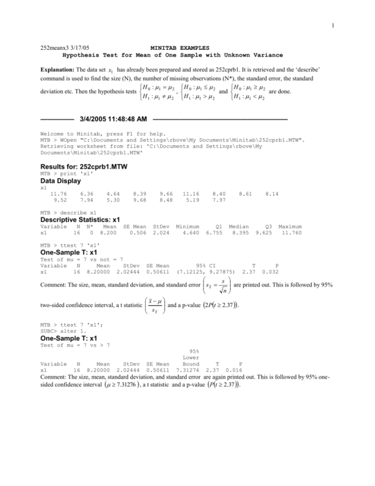
1
252meanx3 3/17/05
MINITAB EXAMPLES
Hypothesis Test for Mean of One Sample with Unknown Variance
Explanation: The data set x1 has already been prepared and stored as 252cprb1. It is retrieved and the ‘describe’
command is used to find the size (N), the number of missing observations (N*), the standard error, the standard
 H :    2  H 0 : 1   2
H :    2
deviation etc. Then the hypothesis tests  0 1
, 
and  0 1
are done.
 H 1 : 1   2  H 1 : 1   2
 H 1 : 1   2
————— 3/4/2005 11:48:48 AM ————————————————————
Welcome to Minitab, press F1 for help.
MTB > WOpen "C:\Documents and Settings\rbove\My Documents\Minitab\252cprb1.MTW".
Retrieving worksheet from file: 'C:\Documents and Settings\rbove\My
Documents\Minitab\252cprb1.MTW'
Results for: 252cprb1.MTW
MTB > print 'x1'
Data Display
x1
11.76
9.52
6.36
7.94
4.64
5.30
8.39
9.68
9.66
8.48
11.16
5.19
8.40
7.97
8.61
8.14
MTB > describe x1
Descriptive Statistics: x1
Variable
x1
N
16
N*
0
Mean
8.200
SE Mean
0.506
StDev
2.024
Minimum
4.640
Q1
6.755
Median
8.395
Q3
9.625
Maximum
11.760
MTB > ttest 7 'x1'
One-Sample T: x1
Test of mu = 7 vs not = 7
Variable
N
Mean
StDev
x1
16 8.20000 2.02444
SE Mean
0.50611
95% CI
(7.12125, 9.27875)
T
2.37
P
0.032

s 
 are printed out. This is followed by 95%
Comment: The size, mean, standard deviation, and standard error  s x 

n

 x 
 and a p-value 2Pt  2.37  .
two-sided confidence interval, a t statistic 

 sx 
MTB > ttest 7 'x1';
SUBC> alter 1.
One-Sample T: x1
Test of mu = 7 vs > 7
Variable
x1
N
16
Mean
8.20000
StDev
2.02444
SE Mean
0.50611
95%
Lower
Bound
7.31276
T
2.37
P
0.016
Comment: The size, mean, standard deviation, and standard error are again printed out. This is followed by 95% onesided confidence interval   7.31276  , a t statistic and a p-value Pt  2.37  .
2
MTB > ttest 7 'x1';
SUBC> alter -1.
One-Sample T: x1
Test of mu = 7 vs < 7
Variable
x1
N
16
Mean
8.20000
StDev
2.02444
SE Mean
0.50611
95%
Upper
Bound
9.08724
T
2.37
P
0.984
Comment: The size, mean, standard deviation, and standard error are again printed out. This is followed by 95% onesided confidence interval   9.08724  , a t statistic and a p-value Pt  2.37  .
Hypothesis Test for Mean of Two Samples with Unknown Variance
Explanation: The data sets x1 and x2 already have been prepared and stored as
2d.mtb. They are retrieved and a 95% confidence interval is taken. Then the
H :   2
hypothesis test  0 1
is done. The intention here was to do a test with a
 H1 : 1   2
significance level of 10%. Since the p-value was 7% (below 10%), we reject the
null hypothesis. For illustration, the opposite test was also done. Note the
high p-value.
Minitab Output:
Worksheet size: 100000 cells
MTB > Retrieve 'C:\MINITAB\2D.MTW'.
Retrieving worksheet from file: C:\MINITAB\2D.MTW
Worksheet was saved on 9/10/1999
MTB > print 'x1''x2'
Comment: Note that n1  n2  2  16  16  2  30 would be
the number of degrees of freedom that we would use
if we were assuming equal variances.
Data Display
Row
1
2
3
4
5
6
7
8
9
10
11
12
13
14
15
16
x1
9.22
6.14
7.14
5.65
7.64
8.63
7.44
8.63
10.11
5.85
12.29
4.86
10.98
8.72
9.72
8.13
x2
7.01
5.35
4.59
6.03
10.85
8.08
7.91
6.16
6.14
11.99
6.67
5.64
6.97
4.66
6.84
8.75
3
MTB > twosamplet 'x1''x2';
SUBC> alter 1.
Two Sample T-Test and Confidence Interval
Twosample T for x1 vs x2
N
Mean
StDev
x1 16
8.20
2.03
x2 16
7.10
2.05
Comment: This is a test of
H 0 : 1   2 against H 1 : 1   2
SE Mean
0.51
0.51
95% C.I. for mu x1 - mu x2: ( -0.38,
T-Test mu x1 = mu x2 (vs >): T= 1.52
2.57)
P=0.070
DF= 29
Comment: Note the reduced number
of degrees of freedom.
MTB > twosample t 'x1''x2';
SUBC> alter -1.
Two Sample T-Test and Confidence Interval
Twosample T for x1 vs x2
N
Mean
StDev
x1 16
8.20
2.03
x2 16
7.10
2.05
SE Mean
0.51
0.51
95% C.I. for mu x1 - mu x2: ( -0.38,
T-Test mu x1 = mu x2 (vs <): T= 1.52
© 2005 Roger Even Bove
Comment: This is a test of
H 0 : 1   2 against H 1 : 1   2
2.57)
P=0.93
DF= 29
Comment: notice the gigantic pvalue.