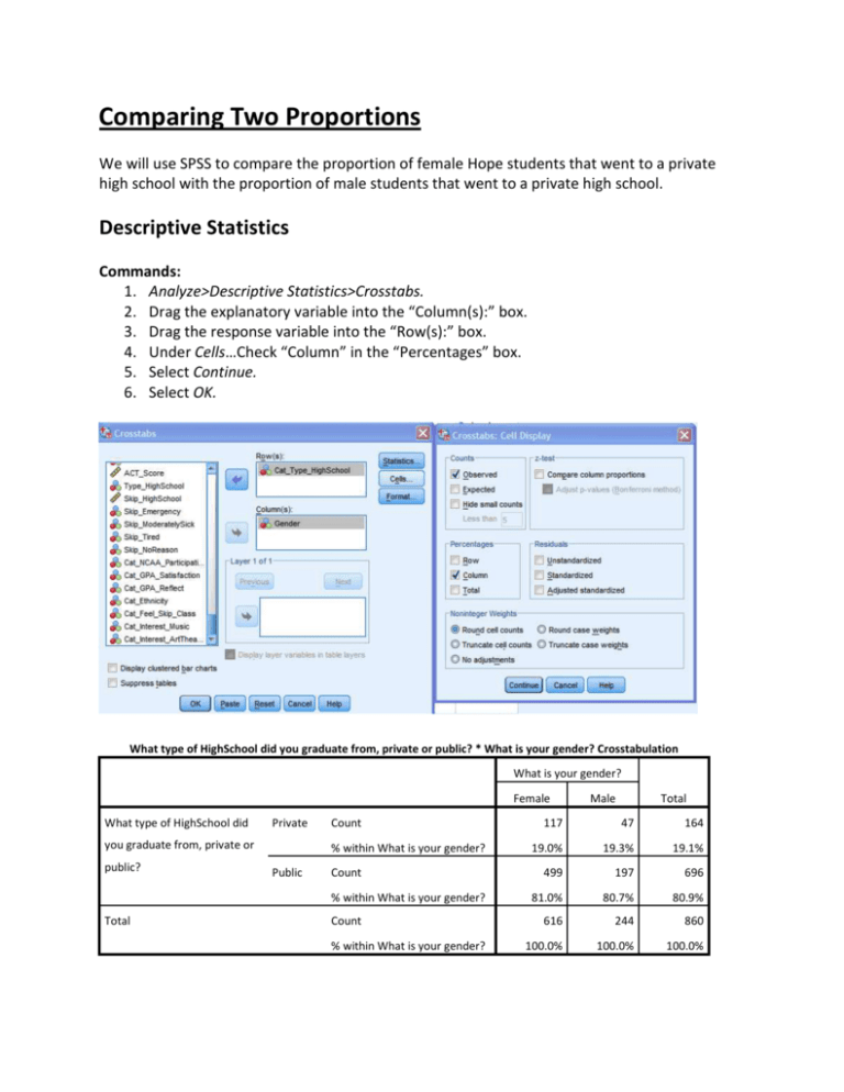
Comparing Two Proportions
We will use SPSS to compare the proportion of female Hope students that went to a private
high school with the proportion of male students that went to a private high school.
Descriptive Statistics
Commands:
1. Analyze>Descriptive Statistics>Crosstabs.
2. Drag the explanatory variable into the “Column(s):” box.
3. Drag the response variable into the “Row(s):” box.
4. Under Cells…Check “Column” in the “Percentages” box.
5. Select Continue.
6. Select OK.
What type of HighSchool did you graduate from, private or public? * What is your gender? Crosstabulation
What is your gender?
Female
What type of HighSchool did
Private
you graduate from, private or
public?
Count
% within What is your gender?
Public
Count
% within What is your gender?
Total
Count
% within What is your gender?
Male
Total
117
47
164
19.0%
19.3%
19.1%
499
197
696
81.0%
80.7%
80.9%
616
244
860
100.0%
100.0%
100.0%
Graphs
Commands:
1. Graphs>Chart Builder>Bar.
2. Drag the stacked bar to the upper window.
3. Drag the explanatory variable to the “X-Axis” box.
4. Drag the response variable to the “Stack: set color” box.
5. Under Statistic: choose Percentage().
6. Under Set Parameters… choose Total for Each X-Axis Category.
7. Select Continue.
8. Select Apply.
9. Select OK.
Inference
Commands:
1. Analyze>Descriptive Statistics>Crosstabs.
2. Drag the explanatory variable into the “Column(s):” box.
3. Drag the response variable into the “Row(s):” box.
4. Under Statistics…Check “Chi-Square.”
5. Select Continue.
6. Select OK.
This box gives us the p-value of .928 (shown in red). The p-value is in the “Pearson Chi-Square”
row and “Asymp. Sig. (2-sided)” column. Note that it is 2 sided.
Chi-Square Tests
Value
Pearson Chi-Square
Continuity Correction
Likelihood Ratio
Exact Sig. (2-
Exact Sig. (1-
sided)
sided)
sided)
a
1
.928
.000
1
1.000
.008
1
.928
.008
b
df
Asymp. Sig. (2-
Fisher's Exact Test
.924
Linear-by-Linear Association
.008
N of Valid Cases
860
1
.928
a. 0 cells (.0%) have expected count less than 5. The minimum expected count is 46.53.
b. Computed only for a 2x2 table
.499
Applet
After you have found descriptive measures, you may take that information and use it in the
Theory-based applet. In fact, SPSS does compute confidence intervals for the difference in
proportions, so if you want this you should use the applet. Below are the graphs, p-value and
confidence interval for our example.
Comparing Two Means
We will use SPSS to compare the average age of female Hope students with the average age of
male Hope students.
Descriptive Statistics and Inference
Commands:
1.
2.
3.
4.
Analyze>Compare Means>Independent-Samples T Test…
The “Test Variable” is the response variable (which should be quantitative).
The “Grouping Variable” is the explanatory variable (which should be categorical).
Define Groups… to indicate to SPSS which two groups are being compared. In the box
“Group1,” type in the variable value (as it appears in “Data View”) for the first group
(i.e.: “0”). In the box “Group 2,” type in the variable value (as it appears in “Data
View”) for the second group (i.e.: “1”). Select Continue.
Group Statistics
What is your gender?
What is your age?
N
Mean
Std. Deviation
Std. Error Mean
Female
643
20.1213
1.67655
.06612
Male
259
20.2355
1.30982
.08139
Independent Samples Test
Levene's Test
for Equality of
Variances
t-test for Equality of Means
95% Confidence
Interval of the
Sig.
F
What is
Equal
.004
Sig.
.948
t
-.982
df
(2-
Mean
Std. Error
tailed)
Difference
Difference
Difference
Lower
Upper
900
.326
-.11421
.11629
-.34245
.11402
-1.089 604.998
.276
-.11421
.10486
-.32015
.09172
your age? variances
assumed
Equal
variances
not
assumed
In red above are the standardized statistic (t-statisitc), the 2-sided p-value, our observed
statistic (the difference in means) and a 95% confidence interval.
Note: SPSS will always give the two-sided p-value. To get the one-sided p-value (assuming that
the sample mean of Group 1 is larger than Group 2 and the alternative hypothesis is such that
the population mean of Group 1 is larger than Group 2), divide the SPSS two-sided p-value in
half.
Graphs
Commands:
1. Graphs>Chart Builder>Boxplot.
2. Drag the simple boxplot to the upper window.
3. Drag the explanatory variable to the “X-Axis” box.
4. Drag the response variable to the “Y-Axis” box.
5. Select OK.
Shown here is side-by-side boxplots are shown of ages for males and females. The open circles
represent potential outliers that are above the upper quartile + 1.5(IQR) and the asterisks
Applet
After you have found descriptive measures, you may take that information and use it in the
Theory-based applet. If you have your data in SPSS in columns right next to each other, you
may also paste that in the applet. Below are the graphs, p-value and confidence interval for our
example.