EE 571 PROBABILITY THEORY AND STOCHASTIC PROCESSSES
FINAL EXAM
Date: 25 Jan 2005
Duration: 150 min.
1-) The random process X(t) is defined as X (t )  u (t   ) , where α is a random variable
uniformly distributed in (0, T) and
t0
t0
(a) Determine the autocorrelation function RXX (t1 , t2 )  E{ X (t1 ), X (t2 )} of X(t).
(b) Sketch the following cross-sections of RXX (t1 , t2 )
1
u (t )  
0
(i) RXX (t , t )
(ii) RXX (t1 , t2  T / 2)
j ωt
2-) Consider the random process X (t )  Ae , where A is a complex constant, ω is a
random variable with pdf fω ( ) .
(a) Find the autocorrelation function of X(t) in terms of fω ( ) .
(b) Show that the power spectral density of X(t) is given by
S XX ( )  2 A f ω ( ) .
2
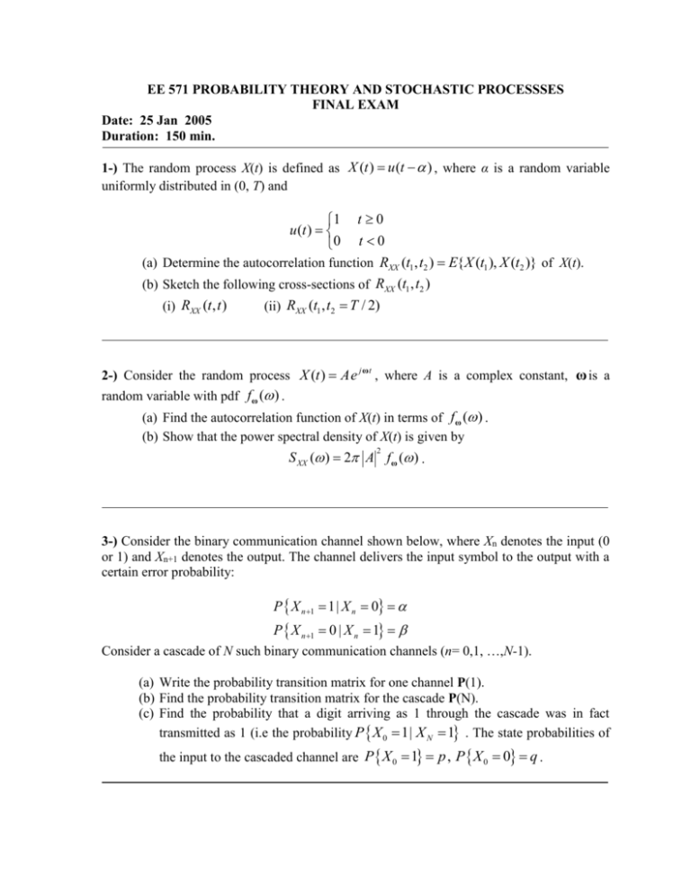
3-) Consider the binary communication channel shown below, where Xn denotes the input (0
or 1) and Xn+1 denotes the output. The channel delivers the input symbol to the output with a
certain error probability:
P  X n 1  1| X n  0  
P  X n 1  0 | X n  1  
Consider a cascade of N such binary communication channels (n= 0,1, …,N-1).
(a) Write the probability transition matrix for one channel P(1).
(b) Find the probability transition matrix for the cascade P(N).
(c) Find the probability that a digit arriving as 1 through the cascade was in fact
transmitted as 1 (i.e the probability P  X 0  1| X N  1 . The state probabilities of
the input to the cascaded channel are P  X 0  1  p , P  X 0  0  q .
0
1-α
0
β
Xn
Xn+1
α
1
1
1-β
4-) Consider a homogeneous Poisson process X(t) such that E{X(9)}=18.
(a) Find the mean and variance of X(8).
(b) Find P  X (2)  3 .
(c) Find P  X (4)  5 | X (2)  3. (Hint: use the fact that the Poisson process has
independent increments)
5-) A LTI continuous-time system has impulse response
e4t
h(t )  
0
t 0
t 0
The input to the system X(t) is a random process with autocorrelation RXX ( )  e
(a) Find the power spectral density SYY ( f ) of the output Y(t) .
(b) Find the average power of the output.
2 
.
SOLUTION
1-) (a)
RXX (t1 , t2 )  E u (t1  α ) u (t2  α )  

 u (t
1
  ) u (t2   ) f α ( )d

T
1
  u(t1   ) u(t2   ) d
T 0
0
 t1

=  tT2
T
 1
t1  0 or t2  0
0  t1  T t2 >t1
0  t2  T t1 >t2
t1 , t2 >T
(c) (i)
0

RXX (t , t )   Tt
1

t0
0t T
t T
1
t
T
(ii)
 Tt1

RXX (t1 , t2  T / 2)   12
0

t1  T / 2
t1  T / 2
t1  0
1/2
T/2
2-) (a)
RXX ( )  E  X * (t ) X (t   )  E  A*e  j ω t Ae j ω (t  ) 
 A E e j ω   A
2

2
e

j 
f ω ( )d 
t
(b)
RXX ( ) in terms of the power spectral density is
1
RXX ( ) 
2

S
XX
( )e j  d

Comparing with the expression in part (a), the uniqueness property of
Fourier transforms gives
S XX ( )  2 A fω ( )
2
3-) (a)
 
1  
P(1)  
1   
 
(b) From lecture notes
P( N )  P(1) N 
1
 
(c)
P  X 0  1| X N  1 
    (1     ) N

N
    (1     )
   (1     ) N 

   (1     ) N 
P  X N  1| X 0  1 .P{ X 0  1} P11 (0, N ). p1 (0)

P{ X N  1}
p1 ( N )
where P11 (0, N ) is the transition probability
   (1     ) N
 
The state probabilities are
p1 (0)  p
p1 ( N )  P01 (0, N ). p0 (0)  P11 (0, N ). p1 (0)
P11 (0, N ) 

   (1     ) N
   (1     ) N
q
p
 
 

 p q

( p  q) 
(1     ) N
 
 
p1 ( N ) 
p  q 1

P  X 0  1| X N  1 
[   (1     ) N ] p
  (  p   q)(1     ) N
4-) (a) E{X(t)}= λt = 18
λ= 18/9 =2
t=9
E{X(8)}= 8×2 = 16
Var{X(8)}= λt = 16
(t )k  t 3 (4)k 4 4
P  X (2)  3  
e 
e e [1  1!4  162!  64
3! ]  0.4335
k 0 k !
k 0 k !
3
(b)
(c)
Let Y  X (2) , Z  X (4)  X (2)  X (4)  Y
X (4)  5
 Z Y  5 ,
 P Z  Y  5 | Y  3 
P Y  k  
4k 4
e
k!
Y and Z are independent Poisson random variables.
P Z  Y  5, Y  3
P Y  3
P Z  n 
and
4n 4
e
n!

P Y  k , Z  n 
4n  k
k 0 n 0 n !k !
3 5 k
3 5 k
P Z  Y  5, Y  3   P Y  k , Z  n  e 8 
k 0 n 0
2
 5 4n 4 4n 1 3 4n  2
4n 3 
 e   



 n 0 n ! n 0 n ! n 0 2(n !) n 0 6(n !) 
 0.1705
8
 P Z  Y  5 | Y  3 
0.1705
 0.3933
0.4335
5-) (a)
SYY ( f )  S XX ( f ) H ( f )

2

H ( f )   h(t )e  j 2 ft dt   e  (4 j 2 f )t dt 
0
0

S XX ( f )   e
0
2 
e  j 2 f  d 
1
4  j 2 f
4
4  (2 f ) 2



4
1
 SYY ( f )  
2
2
 4  (2 f )  16  (2 f ) 
4n  k 8
e
n !k !
(b)

E{Y (t )} 
2
S
YY
( f )df
s  j 2 f
 E{Y (t )} 
2

j
c ( s )c (  s )
ds
2 j  j d ( s )d ( s )
1


 c( s ) c(  s )
2
2
 4  1  
SYY ( s )  



2
2
 4  s  16  s   (2  s)(4  s)   (2  s)(4  s)  d ( s) d (  s)
c( s )  2  c0  2 c1  0
d ( s)  s 2  6s  8
E{Y 2 (t )} 

d0  8
d1  6
c12 d 0  c02 d 2
4
1


2d 0 d1d 2
2  8  6 24
d2  1