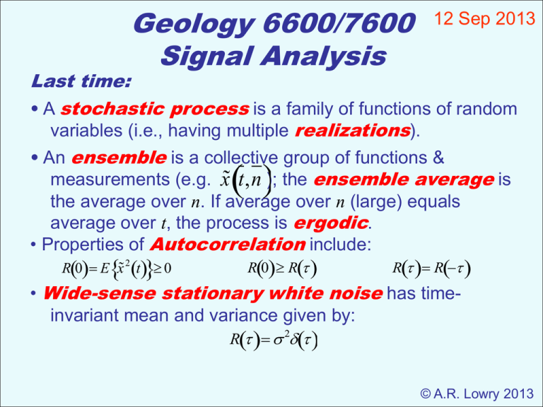
Geology 6600/7600
Signal Analysis
12 Sep 2013
Last time:
• A stochastic process is a family of functions of random
variables (i.e., having multiple realizations).
• An ensemble is a collective group of functions &
measurements (e.g. x˜ t,n ); the ensemble average is


the average over n. If average over n (large) equals
average over t, the process is ergodic.
• Properties of Autocorrelation include:
 
R0 R 
R0 E x˜ 2 t  0
R  R 
• Wide-sense stationary white noise has timeinvariant mean and variance given by:


R   2  
© A.R. Lowry 2013

A random process is Nearly Wide-Sense Stationary
if the mean varies as a function of time, Ex˜t t,
but the autocovariance is time-invariant:
Cxx   C  Ct1,t2 

(Note that we’ve introduced a new notation here: Cxx() is
the autocovariance of the random process x˜ t .)

In this case we can form a new random variable,
z˜t x˜ t t, with z t Ex˜t t 0. Since the mean is
~
constant for z,
it’s a stationary process
with Rzz() = Czz().


The Cross-Correlation for two wide-sense stationary
processes is given by:
Rxy   Ex˜t   y˜t
Properties:
(1) Even:

(2) Bounded:
Rxy() = Ryx(–)
(Show as exercise!)
Rxy2() ≤ Rxx(0)Ryy(0)
(*Note that cross-correlation is among the most widely-used
tools in seismology! Including seismic interferometry
[e.g., “ambient noise” methods], NMO correction,
automated picking of travel times, & much more)
Example: What is the autocorrelation of a linear combination
of two random variables? Consider e.g.:
z˜t ax˜ t by˜ t
The autocorrelation:
Rzz   
(Exercise…)



E ax˜ t    by˜ t   ax˜ t by˜ t
 a 2 Rxx   abRyx   abRxy   b 2 Ryy  
If the random variables are uncorrelated and zero-mean
(i.e., Rxy() = 0!), then

Rzz   a 2 Rxx   b2 Ryy  
These relations hold for discrete as well as continuous
random variables…

Discrete-time Processes can be expressed similarly:
We’ll use the notation:
x˜ n for sampled x˜ t 
Mean:

n  Ex˜ n
Autocorrelation:

Rn1,n2   Ex˜n1x˜n2 
Autocovariance:



Cn1,n2   E x˜ n1 n1x˜ n2  n2 


Rn1,n2  n1n2 
For a wide-sense stationary (WSS) process
(here l = n1 – n2 is lag, analogous to continuous ):

Ex˜n 
Rn1,n2   Rl  Rxx l
And for a white noise process:

Cxx
l   l  Rxx l if
2
 = 
0
Rxy n1,n2   Rxy l
1, l  0
 l  
0 l  0
Ergodic Processes:
Ergodicity requires that time averages equal ensemble
averages (i.e. expected values across time for one
member of an ensemble equal expected values at one
given time across ensembles).
Weakly WSS ergodic processes have properties:
1)


1
˜T  E lim
E

T  2T
Ensemble
Average

2)
3)


x˜tdt


T
Time
Average
T

Any
Realization
T




1
˜
ERT  E lim
x˜ t   x˜ tdt R 


T  2T T


˜T &VR˜T 0 as T 
V
Example of a non-ergodic process: let
x˜ t a˜, Ea˜ , Va˜  2
Then:
1
˜T  lim

T  2T

T
 a˜dt  a˜
T
˜T  Ea˜ 
E
So the first
 condition is satisfied. However
˜T Va˜  2
V

does not go to zero as T , so the third condition is not
satisfied.

We now have the basic working formulae:
1
˜T  lim

T  2T

1
R˜xx   lim
T  2T
1
R˜xy   lim
T  2T

T
 x˜tdt
T
T
 x˜t   x˜tdt
T
T
 x˜t   y˜tdt
T
So in the case of ergodic signals, the auto- and
cross-correlation functions can be expressed as

convolutions
of x with itself and with y respectively:
 f  g   f tg  tdt

Hence:
R˜xx   x˜t x˜t 


R˜xy   x˜t y˜t 
So how does all of this relate to the power spectrum?
(Hint: Convolution in the “spectral domain”— I.e., after
Fourier transformation— is a simple multiplication…)
The Auto-Power Spectrum of a random variable is
given by the Wiener-Khinchin relation:
Sxx 

 R  e
xx

i
d


1
Rxx  
Sxx e i d
2 
Hence thepower spectrum is the Fourier Transform of the
correlation function!

Grokking the Fourier Transform:
Power spectra and the Fourier Transform to the frequency
domain are fundamental to signal analysis, so you should
spend a little time familiarizing yourself with them. For the
following functions, I’d like you to first evaluate the integral
by hand, & then calculate and plot the Fourier transform
using Matlab.
(Send me by class-time Tuesday Sep 23).
1) Autocorrelation of a discrete-time WSS white noise
process (use 2 = 3)
2) A constant (use a = 3)
3) A cosine function (use amplitude 1; )
4) A sine function (as above)
5) A box function (0 on [–,–/2] & [/2,]; 1 on [–/2,/2])
As a shorthand for the forward and inverse Fourier
transform, we will use e.g.:
Rxx   Sxx 
Some properties of the Fourier transform: Recalling Euler’s
relation, e–it = cos(t) – isin(t), the FT of an even
function will always be even (and real), and the FT of an
 will always be odd and imaginary.
odd function
Hence, because the autocorrelation function Rxx is real
and even, the autopower spectrum Sxx will always be
real and even as well!
Note however this also implies that the power spectrum
does not contain any phase information about the
signal…