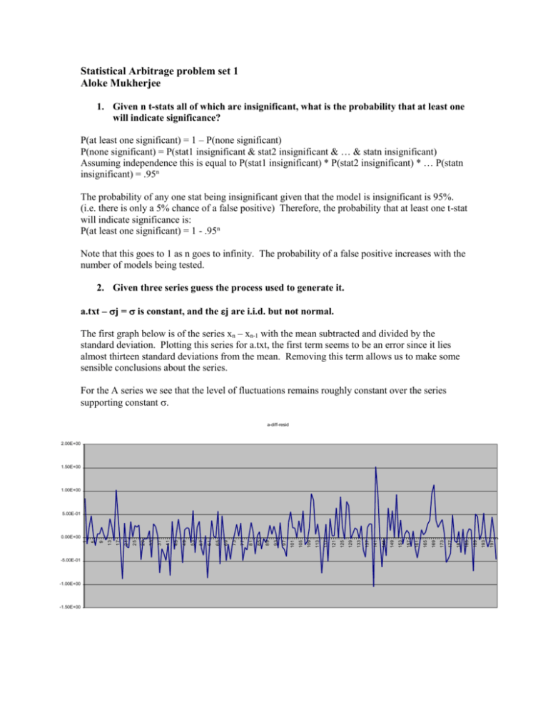
Statistical Arbitrage problem set 1
Aloke Mukherjee
1. Given n t-stats all of which are insignificant, what is the probability that at least one
will indicate significance?
P(at least one significant) = 1 – P(none significant)
P(none significant) = P(stat1 insignificant & stat2 insignificant & … & statn insignificant)
Assuming independence this is equal to P(stat1 insignificant) * P(stat2 insignificant) * … P(statn
insignificant) = .95n
The probability of any one stat being insignificant given that the model is insignificant is 95%.
(i.e. there is only a 5% chance of a false positive) Therefore, the probability that at least one t-stat
will indicate significance is:
P(at least one significant) = 1 - .95n
Note that this goes to 1 as n goes to infinity. The probability of a false positive increases with the
number of models being tested.
2. Given three series guess the process used to generate it.
a.txt – j =  is constant, and the j are i.i.d. but not normal.
The first graph below is of the series xn – xn-1 with the mean subtracted and divided by the
standard deviation. Plotting this series for a.txt, the first term seems to be an error since it lies
almost thirteen standard deviations from the mean. Removing this term allows us to make some
sensible conclusions about the series.
For the A series we see that the level of fluctuations remains roughly constant over the series
supporting constant .
a-diff-resid
2.00E+00
1.50E+00
1.00E+00
5.00E-01
-5.00E-01
-1.00E+00
-1.50E+00
197
193
189
185
181
177
173
169
165
161
157
153
149
145
141
137
133
129
125
121
117
113
109
105
97
101
93
89
85
81
77
73
69
65
61
57
53
49
45
41
37
33
29
25
21
17
9
13
5
1
0.00E+00
The histogram of the series compared with the normal pdf below shows that the distribution of
the j is not normal. It is much more peaked at the center. This is visible in the residual time
series’ generally small fluctuations. Further confirmation is given by the kurtosis which is greater
than three and has a t-statistic greater than two allowing us to reject the normal hypothesis for the
residuals of A.
b.txt -  is constant, and the j are i.i.d. standard normal.
b-diff-resid
2.50E+00
2.00E+00
1.50E+00
1.00E+00
5.00E-01
-5.00E-01
-1.00E+00
-1.50E+00
-2.00E+00
-2.50E+00
Again, the first sample in this series alters all the subsequent analysis, it lies greater than five
standard deviations from the mean. Discarding this sample produces a series with a constant
level of fluctuation, supporting the hypothesis of constant . The normalized histogram fits the
standard normal distribution well and the kurtosis lies within 1.4 standard deviations of its
expected value.
196
191
186
181
176
171
166
161
156
151
146
141
136
131
126
121
116
111
106
96
101
91
86
81
76
71
66
61
56
51
46
41
36
31
26
21
16
6
11
1
0.00E+00
c.txt - The j are i.i.d. standard normal, but j depends on j in a “smooth” fashion: it has
some consistent trend through the data sample but it does not vary randomly.
The normalized residuals of C clearly show a reducing level of fluctuations. Stratifying the
sample into subgroups of twenty and plotting the standard deviations of each clearly shows a
linear downward trend in j. This is shown in the second graph below.
3. IBM daily price and returns.
Daily holding period return is defined as the return you would’ve earned if you’d bought the
stock at the last valid price before today and held till today. The last valid price can be up to ten
days earlier.
Holding period return: R = (Today/Last) – 1
This is equivalent to % price change if the last price was from the previous trading day and there
are no adjustment factors. This is roughly equivalent to log price change but only to order R.
IBM return series - 2000-2005
0.15
0.1
0.05
0
-0.05
-0.1
-0.15
1462
1401
1340
1278
1217
1156
1097
1036
975
913
852
791
732
671
610
548
487
426
367
306
245
183
122
61
1
-0.2
The IBM return series is not normal. Looking at the graph of price changes we can
clearly see that volatility has changed over time, that small returns are far more likely and
that large swings occur more often than would be possible if returns were normally
distributed. These observations are confirmed by a comparison of the distribution with
the normal PDF. It clearly shows that IBM’s returns distribution has a higher central
peak and fatter tails. The kurtosis is high enough to allow the normal hypothesis for
IBM’s returns to be safely rejected.
The IBM return series does not seem to be i.i.d. The first correlogram below shows that at
some lags the IBM return autocorrelation exceeds the 95% interval. For comparison,
correlograms were computed for three series of i.i.d normal random variables of the same length
as the IBM return series. Only at one lag in one of the series does the autocorrelation exceed the
95% interval. By comparison the IBM return series exceeds the 95% interval three times – at lags
of one, four and eighteen days.
The third graph below compares the correlograms for the first and second halves of the series.
The first half of the series closely mirrors the autocorrelation for the entire series. Interestingly,
the second half of the series does not reject the i.i.d. hypothesis. This shows that the
autocorrelation is not necessarily stationary for this series.
4. Fit a mean-reverting model to the federal funds rate over the past thirty
years.
The data from CRSP includes dates with no data. These were assumed to be the same as
the previous days data. To fit the model xj = α+βxj−1+σεj we regress xj on xj-1 using
Excel’s regression function. This yields the following statistics:
SUMMARY OUTPUT
Regression Statistics
Multiple R
0.994669072
R Square
0.989366562
Adjusted R Square
0.9893652
Standard Error
0.379646306
Observations
7810
ANOVA
df
Regression
Residual
Total
Intercept
X Variable 1
SS
104708.4384
1125.37733
105833.8157
MS
104708.4384
0.144131318
Coefficients Standard Error
0.035284897
0.008838429
0.994669072
0.00116699
t Stat
3.992213677
852.3376296
1
7808
7809
From the regression we have the following parameter values:
α = 0.0353
β = 0.9947
σ = 0.3796
If this were a O-U type model (xj = κ (θ - xj−1) + σεj), this would yield parameters:
κ (speed of mean-reversion) = 1 – β = 0.00533 (1/κ= 187.5 days)
θ (long-run average) = α/κ = 6.62%
This model does not fit the data well since the residuals are far from the standard normal
distribution. The residuals exhibit time-varying volatility, variations far beyond what could
occur under a normal distribution (one greater than twenty standard deviations) and excess
kurtosis. This is illustrated below in a graph of the residuals vs. time and a histogram of the
residual values compared with the standard normal pdf.
distribution of residuals from fed fund regression
1
0.9
0.8
0.7
0.6
0.5
0.4
0.3
0.2
0.1
0
-5.25
-4.75
-4.25
-3.75
-3.25
-2.75
-2.25
-1.75
-1.25
-0.75
-0.25
0.25
normalized histogram
0.75
1.25
1.75
2.25
2.75
3.25
3.75
standard normal pdf
4.25
4.75
5.25