Two Material Thermal Stress Model (draft 3 2/19/06)
Introduction
Design tasks often involve parts made of more than one material. Sometimes the materials are
bonded together and at other times they are not. Assembled parts may look like they consist of
bonded parts simply because appear to be touching. However, analysis software assumes that
adjacent parts are not bonded or even in contact unless the user specifically establishes such
relations. To illustrate these concepts consider the common elementary physics experiment of
uniformly heating two bonded beams made of materials having different coefficients of thermal
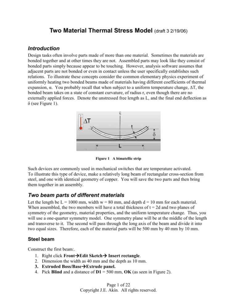
expansion, α. You probably recall that when subject to a uniform temperature change, ∆T, the
bonded beam takes on a state of constant curvature, of radius r, even though there are no
externally applied forces. Denote the unstressed free length as L, and the final end deflection as
δ (see Figure 1).
Figure 1 A bimatellic strip
Such devices are commonly used in mechanical switches that are temperature activated.
To illustrate this type of device, make a relatively long beam of rectangular cross-section from
steel, and one with identical geometry of copper. You will save the two parts and then bring
them together in an assembly.
Two beam parts of different materials
Let the length be L = 1000 mm, width w = 80 mm, and depth d = 10 mm for each material.
When assembled, the two members will have a total thickness of t = 2d and two planes of
symmetry of the geometry, material properties, and the uniform temperature change. Thus, you
will use a one-quarter symmetry model. One symmetry plane will be at the middle of the length
and transverse to it. The second will pass through the long axis of the beam and divide it into
two equal sizes. Therefore, each of the material parts will be 500 mm by 40 mm by 10 mm.
Steel beam
Construct the first beam:.
1. Right click FrontEdit Sketch Insert rectangle.
2. Dimension the width as 40 mm and the depth as 10 mm.
3. Extruded Boss/BaseExtrude panel.
4. Pick Blind and a distance of D1 = 500 mm, OK (as seen in Figure 2).
Page 1 of 22
Copyright J.E. Akin. All rights reserved.
Figure 2 Sketch and extrude a strip
Now that you have built the first beam body, assign it the material property of steel.
1. Right click on Materials <none selected> Edit Material.
2. In the Materials Editor select the material desired, OK.
3. Verify that the part now shows the selected material name, see Figure 3.
4. FileSave as filename steel_beam.sldprt.
Figure 3 Assign and verify a material
Copper beam
Open a new (second) part. Repeat the processes above except select copper as the material and
save it with the filename copper_beam. Use WindowTile Horizontally to see both parts, such
as seen in Figure 4.
Part assembly and geometric mating
Now open a new assembly:
1. Use NewAssemblyOK.
2. In the Insert Component panel click on the steel beam in its window and drag it to the
assembly window. As the first part it will be fixed in the view and other parts will move
relative to it.
3. Click on the copper beam part and drag it into the assembly window. These steps are
summarized in Figure 5.
Page 2 of 22
Copyright J.E. Akin. All rights reserved.
Next you need to carry out the geometric mating of the different materials so that the surfaces
that may be bonded in the finite element analysis are touching in the assembly:
1. Select the Mate icon.
2. In the Mate panel pick concentric as the Standard Mate.
3. Select the long bottom edge of the copper and the long top edge of the steel as the Mate
selections, OK.
4. In the Mate panel pick concentric as the Standard Mate.
5. Select the short bottom front edge of the copper and the short top front edge of the steel
as the Mate selections, OK. These steps are summarized in Figure 6.
6. Finally, FileSave as file name copper_steel.sldasm.
Figure 4 View both parts in tiled windows
Page 3 of 22
Copyright J.E. Akin. All rights reserved.
Figure 5 Insert both parts into a new assembly
Figure 6 Geometrically mate the common faces
Before leaving the assembly, note in Figure 7, that the copper part was placed on top of the steel
part. That should give you a hint on the deflection directions that will be computed in the
CosmosWorks study.
Page 4 of 22
Copyright J.E. Akin. All rights reserved.
Figure 7 The mated assembly before entering CosmosWorks
Estimated deflection results
Before building a full computer model you should try to estimate what to expect as an answer.
As the assembly was built, the copper was on top. Since it has a higher coefficient of thermal
expansion the top will get longer that the bottom. If they are bonded then beam should bend
away from the copper. If bonded there will be a common axial extension, which is less than the
free thermal expansion of the copper, but more than the free expansion of the steel. An equal
and opposite set of internal bonding forces are developed at the common (equilibrium) extension.
The classic handbook “Roark’s Formulas for Stress and Strain” [1] gives the beam theory
solution for the deflections and stresses for a bimetallic strip (neglecting Poisson’s ratio included
here). The maximum deflection for equal thickness material layers reduces to:
δY = 6(αS – αC)(T-T0)(L2) / (t2 K1), K1 = 14 + (ES / EC) + (EC / ES).
For the given data: K1 = 16.433, (T-T0) = 280 C, (αS – αC) = - 1.1e-5 1/C, L = 0.5 m, and t = 0.01
m which yields δY = 0.0281 m.
CosmosWorks thermal stress model
Beginning a study
Assume that the mated assembly was stress free at a temperature of 20 C and is to be heated to a
uniform temperature of 300 C. Still in the assembly process, begin a CosmosWorks study.
1. Select the CosmosWorks icon to open its manager panel.
2. Because the assembly has touching faces the Contact/Gaps feature appears.
3. Right click on it and select Bonded touching faces, as in the upper part of Figure 8.
(Later, you will try Free for comparison purposes).
4. Right click on the Part NameStudy
5. In the Study panel give a Study name, pick the static Analysis type, and select a solid
(or shell) Mesh type, OK (see the lower part of Figure 8)
Page 5 of 22
Copyright J.E. Akin. All rights reserved.
Having given a study name and a mesh type you would usually click on the mesh type and assign
material properties. However, that assignment was made within SolidWorks while constructing
the two individual beam parts. Of course, you could edit the imported properties at this point if
you have decided on a different material.
Figure 8 Bond the touching faces and select a solid mesh
Material selections and thermal loading
Remember that the material properties for each beam were selected within SolidWorks. They
have been imported into CosmosWorks and may need to be reviewed or edited. In this problem
you have bonded materials subjected to the same temperature change. Therefore the coefficients
of thermal expansion (actually their difference) are very important and should be double
checked. Assume that has been done.
Identify the thermal loading early in the process through the pull down Properties option (and
not by the usual Temperature panel under Loads/Restraints).
1. Right click on the Study nameProperties.
2. In the Static panel pick Flow/Thermal Effects.
3. Check the Include thermal effects, and pick Uniform temperature.
4. Enter the final temperature value and units and the stress free (zero strain) temperature,
OK. These steps are summarized in Figure 9.
For future reference you should note that the Static panel provides for non-uniform temperature
distributions to be input, or imported from external files.
Restraints
As with any problem, you must prevent the six possible rigid body motions (RBM). That must
be done in a way that does not restrict the thermal motion, unless the true support system does
that. You also need to invoke the two symmetry planes used to reduce the computational costs.
The first (short) symmetry plane restrains rigid body motion in the direction of the long axis of
the beam (i.e. normal to the plane). Since there are multiple points on that restraint plane it will
also prevent RBM about the two coordinate axes lying in that plane (so 3 RBM remain to be
Page 6 of 22
Copyright J.E. Akin. All rights reserved.
Figure 9 Setting properties of a uniform temperature change
addressed). The second (long) symmetry plane must also prevent displacement normal to it, and
thus also prevents the third remaining RBM rotation (1 RMB translation remains). Finally, one
point must be restrained to eliminate the remaining possible RBM (in the direction parallel to the
corner formed by the two symmetry planes). Any point in the assembly could be picked and all
computed motions in this last direction will be computed relative to that chosen point. The most
logical point to chose is in the corner junction of the first two restraint planes, and at the interface
of the two materials at the center of the beam.
Those three restraint operations are outlined in Figure 10. The basic steps are:
1. Right click on Loads/RestraintsRestraintsRestraint panel.
2. Pick the on a flat face Type with zero normal Displacement and use the symmetry plane
as the Selected Entities, OK.
3. Right click on Loads/RestraintsRestraintsRestraint panel.
4. Use the corner vertex as the Selected Entities, and fixed as the Type. (Actually, you only
needed to fix the displacement parallel to the intersection line of the first two restraint
planes because two of the point restraints are already done.)
Mesh control
You should expect the temperature change to cause a bonded beam to curve. Therefore bending
stresses will develop. A crude mesh will probably give a reasonably accurate displacement
calculation. However, to get accurate bending stress recovery you need at least 5 to 6 layers of
elements through the thickness of each material. That requires mesh control on each of the four
faces sharing the thickness dimension. Bending fiber stresses are most likely to be large on the
top and bottom layer of each material. Thus they need a good surface mesh too. You can either
lower the average element size to get that and/or manually control the element sizes on those
three surfaces:
Page 7 of 22
Copyright J.E. Akin. All rights reserved.
1. Right click on MeshMesh Control.
2. In the Mesh Control panel, of Figure 11, select both parts in the assembly as the
Selected Entities and check use same element size.
3. Examine the default element size and reduce it 3 mm for an initial mesh.
4. Right click on MeshCreate, then MeshShow mesh.
Figure 10 Preventing all six rigid body motions
Mechanical Loading
Remember that there are no external mechanical loads to be applied here, and the uniform
temperature change has all ready been addressed.
Page 8 of 22
Copyright J.E. Akin. All rights reserved.
Displacements solution
There are many displacement degrees of freedom in this mess and most are wasted since there
will be little change in displacements through the width, w. While you should get good
deflection results the three elements through each material thickness may not give good stress
estimates. (A shell model, in plane stress, probably would have been more accurate and had
much fewer equations to solve.) Now start the equation solver with Study name Run in the
manager panel.
Figure 11 Applying uniform volumetric element sizes
Post-processing
Displacement results
A look at the deformed shape shows the shape that was expected due to the higher thermal
expansion coefficient of the copper. The overall displacement size (un-magnified) is large
compared to the total beam thickness. That would usually mean that you should consider a
geometrically non-linear “large deflection analysis”, but it might not be justified for this thermal
loading.
Page 9 of 22
Copyright J.E. Akin. All rights reserved.
If the materials had not been bonded you would have just axial (UZ) displacements. Looking at
them in detail, as seen in Figure 12, you see that component is always positive, but decreasing
from top to bottom (from copper to steel).
Figure 12 The deformed shape and its axial components
The total displacements (URES), and the transverse (UY) components, given in Figure 13, are
much larger that the previous axial components. You can create a list of the largest UY
components by zooming in on the region and picking nodes:
1. Right click in the graphics area and select Probe.
2. Select the desired nodes and the component values will be added to the plot (usually this
step is easier if you use MeshShow mesh before Probe), and placed in a list that
appears in the Probe panel.
Page 10 of 22
Copyright J.E. Akin. All rights reserved.
Figure 13 The undeformed assembly, resultant and UY displacement components
Listing and graphing displacements
XXX
Page 11 of 22
Copyright J.E. Akin. All rights reserved.
Page 12 of 22
Copyright J.E. Akin. All rights reserved.
Page 13 of 22
Copyright J.E. Akin. All rights reserved.
Thermal stresses
The stresses in the bimetallic beam should be essentially constant except very close to the free
end. Thus, you need only display the two ends in detail. The mid-span symmetry plane normal
Z-stress component (beam fiber stress) is given in the top of Figure 14, while the bottom of that
figure shows the corresponding results at the free end. The wiggles in the contours imply that
the mesh is too crude near the center bonding plane (which is an important region for this load
state.)
Page 14 of 22
Copyright J.E. Akin. All rights reserved.
Figure 14 The fixed and free end axial fiber stress magnitudes
To view these data in another way display a vector plot on this component (at each end of the
beam):
1. Right click in graphics area, Edit DefinitionVectorLine.
2. Right click in graphics area, Vector plot options, and dynamically control the maximum
vector size, and the percentage of nodes shown (see Figure 15).
Observe that this type of plot does not make obvious the presence of a crude mess.
Page 15 of 22
Copyright J.E. Akin. All rights reserved.
Figure 15 The mid-section and free end axial fiber stress component vectors
At this point (because of Figure 14) you should already expect that this mesh is too crude to rely
upon for stress results. To verify that, consider the free end region von Mises failure criterion
plot of Figure 16. Clearly, the contour lines have many wiggles and the study should be repeated
with a finer mesh and/or a plane stress (shell) mesh. If you look at the deflection and stress plots
in all three coordinate planes (not shown here) you see that this 3D model has mainly a 2D
response. Very little is changing through the 40 mm half width. That also suggests using a shell
model for a refined model. After doing that you could more wisely control a 3D mesh for a final
study.
Page 16 of 22
Copyright J.E. Akin. All rights reserved.
Figure 16 Crude von Mises contours at the free end region
Wiggles is stress contours can also be caused by using the default small deflection theory (as
done here) to obtain a result that seems to be a large deflection result (greater than half the
smallest material or part thickness). Figure 12 suggests that this study should be rechecked, after
the final part revisions, with a large displacement analysis option.
Listing and graphing stresses
CosmosWorks allows the creation of tables and graphs of any component available in the postprocessing graphics options. To display such items you:
1. Display component of interest.
2. Right click in graphics area  List Selected.
3. Pick the surface or (split line) curve.
4. Click on the Update button on List Selected panel. Note that the Sum, Average,
Maximum, and Minimum values are listed along with all the nodal values selected.
5. To display a graph of the selected items click on the Plot button. For a surface you get a
graph (in more or less random order) by node positions. For a line or curve selection you
get a graph versus the non-dimensional position along the curve. You should plan ahead
for such displays by adding split lines to the model where the model edges are not where
you wish to plot the results.
Page 17 of 22
Copyright J.E. Akin. All rights reserved.
Figure 17 Axial stress along top edge
Page 18 of 22
Copyright J.E. Akin. All rights reserved.
Figure 18 Axial stress along bottom beam edge
Page 19 of 22
Copyright J.E. Akin. All rights reserved.
Validation calculations
While you may not trust the current stress results, you should still compare the computed
displacements (which are always more accurate that the computed stress) to the initial
engineering estimate of the maximum deflection. The computed maximum magnitude, in Figure
13 , was about 2.87 mm. The original deflection estimate was δY = 2.81 mm, so the agreement
was surprisingly good.
Large deflection check
CosmosWorks allows a large deflection calculation for solid meshes only. A large deflection
analysis applies an iterative loading and displacement solution loop. In each loop a small part of
the (thermal) loading is added to form a new resultant load. The corresponding displacements
are computed and added to the original positions of the elements’ nodes. The updated element
positions are employed to re-compute the element stiffness matrices. The looping is repeated
about 10 to 20 times to obtain the final displacements and the last set of element stresses. That is
usually called a “geometrically non-linear analysis” (as contrasted to a “materially non-linear
analysis” which is much more complicated).
While some finite element systems have such a free standing option, in CosmosWorks you must
employ a little trick you activate that feature since it was designed to be used with the large
deflection contact analysis. The trick is to select two surfaces, on different components of the
assembly, and have CosmosWorks check for them contacting (an additional and relatively
computationally expensive process). Time is spent checking for a contact you know is extremely
unlikely to occur, but you still get the desired large deflection analysis.
Start a new study
Such an analysis runs about 50-60 times longer that the standard analysis presented above. This
was done, but the process is only outlined here since the changes were quite small and it takes a
long time to run. To use this process you need a new study:
1. Right click on the Assembly nameStudy to get to the Study panel.
2. In the Study panel assign a new Study name, Analysis type, and Mesh type. Before
closing that panel, also pick Properties to get the Static panel.
3. In the Static panelOptions check Large displacement contact, and next select
Flow/Thermal Effects and set the same conditions as in Figure 9.
Some of the above steps are seen in Figure 19.
Figure 19 Starting a large deflection (fake) contact analysis
Page 20 of 22
Copyright J.E. Akin. All rights reserved.
When the assembly opens, you will see that the Contacts/Gaps icon has appeared above the
usual Mesh icon location. The new icon must be used to both bond the touching faces, as before,
but also to pick to potential contact surfaces as a trick to activate the large deflection iterative
solver. To do that:
1. Right click Contact/Gaps, turn on Touching Faces Bonded, and select Define Contact
Pair.
2. When the Contact Pair panel appears, select a surface Type, pick the symmetry end
surface on the copper component (actually any copper surface for a fake contact), rotate
the assembly and pick the free end surface of the steel, respectively as the Selected
EntitiesOK.
The latter two steps are seen in the lower left and lower right parts, respectively of Figure 20.
Figure 20 Bonding the parts and selecting fake contact surfaces
New large deflection solution results
Using the usually solution process, Assembly nameRun (and a slightly cruder mesh) you
eventually get new results for the displacements and stresses. However, they are nearly the same
despite a much longer solution time. The new results are summarized in Figure 21. The bottom
part of that figure shows the cruder mesh used here superimposed on the von Mises contours,
which seem even less useful that from the original study. Thus, this study itself needs to be
redone, with a much finer mesh through the thickness. Make that change, restart the iterative
solution, and go out for a snack break.
Closure
The bonding makes a great difference in the response of any assembly. To see that, you could
reload the assembly and not bond the touching surfaces. The resulting stresses should be zero
and the displacements will only be in the UZ direction (try it).
Page 21 of 22
Copyright J.E. Akin. All rights reserved.
Figure 21 Selected large deflection results
Reference:
1. W.C. Young, R.G. Budynas, Roark’s Formulas for Stress and Strain, 7-th Ed., McGrawHill, New York, 2002.
Page 22 of 22
Copyright J.E. Akin. All rights reserved.