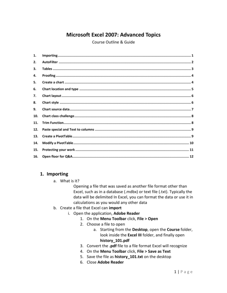
Microsoft Excel 2007: Advanced Topics
Course Outline & Guide
1.
Importing ........................................................................................................................................ 1
2.
AutoFilter ....................................................................................................................................... 2
3.
Tables ............................................................................................................................................. 3
4.
Proofing .......................................................................................................................................... 4
5.
Create a chart ................................................................................................................................. 4
6.
Chart location and type .................................................................................................................. 5
7.
Chart layout .................................................................................................................................... 6
8.
Chart style ...................................................................................................................................... 6
9.
Chart source data............................................................................................................................ 7
10.
Chart class challenge ....................................................................................................................... 8
11.
Trim Function.................................................................................................................................. 8
12.
Paste special and Text to columns .................................................................................................. 9
13.
Create a PivotTable ......................................................................................................................... 9
14.
Modify a PivotTable ...................................................................................................................... 10
15.
Protecting your work .................................................................................................................... 11
16.
Open floor for Q&A....................................................................................................................... 12
1. Importing
a. What is it?
Opening a file that was saved as another file format other than
Excel, such as in a database (.mdbx) or text file (.txt). Typically the
data will be delimited In Excel, you can format the data or use it in
calculations as you would any other data
b. Create a file that Excel can import
i. Open the application, Adobe Reader
1. On the Menu Toolbar click, File > Open
2. Choose a file to open
a. Starting from the Desktop, open the Course folder,
look inside the Excel III folder, and finally open
history_101.pdf
3. Convert the .pdf file to a file format Excel will recognize
4. On the Menu Toolbar click, File > Save as Text
5. Save the file as history_101.txt on the desktop
6. Close Adobe Reader
1|Page
c. Open Excel and import the data
i. Select the file to Import
1. Select the Office button > Open
2. In the Open window, to the right of the Files of type:,
choose All Files (*.*) from the drop down list
3. At the top of the window, to the right of Look In:, select
desktop
4. From the list of files available select and open,
history_101.txt
ii. Setup the Import Wizard
1. In the new Import Wizard window, under Original data
type, select Delimited
2. Click Next
3. In the Step 2 window, under Delimiters, only check Space
4. Click Next
5. In the Step 3 window, under Column data format, select
General
6. Click Finish
7. Note: the data imported contains no formulas or functions
and any cell formatting is now General
iii. Class Challenge
1. Change the column headers to match the data below
2. Adjust the headers to match the data
iv. Delete row 7
1. It is no longer setup to run functions or formulas
d. Save the Excel file
i. Select the Office button > choose Save As > Excel Workbook
ii. Save on the desktop
iii. Name the file history_101.xlsx
2. AutoFilter
a. What is it?
Filtered data displays only the rows that meet criteria that you
specify and hides rows that you do not want displayed. After you
filter data, you can copy, find, edit, format, chart, and print the
subset of filtered data without rearranging or moving it
b. Apply AutoFilter
i. Select cells A2 through J2
ii. On the Ribbon, select Home tab, in the Editing group, select Sort
& Filter, in the menu select Filter
iii. The row of cells previously selected should now have drop down
arrows
c. View records by criteria
2|Page
i. Movie your mouse pointer to the Pass/Fail column header and
select the down arrow
ii. In the new window, uncheck the value Fail (this is the value of the
records you do not want to view)
iii. Click OK
iv. You should now only see the students who passed the class
v. Potentially you could continue to narrow the field of records
viewed by deselecting criteria from other headings
d. To “Clear” the criteria you set for one or more columns
i. Select cells A2 through J2
ii. On the Ribbon, select Home tab, in the Editing group, select Sort
& Filter, in the menu select Clear
e. Remove AutoFilter
i. Select cells A2 through J2
ii. On the Ribbon, select Home tab, in the Editing group, select Sort
& Filter, in the menu select Filter
iii. The row of cells previously using AutoFilter should no longer have
drop down arrows
3. Tables
a. What are they?
A table is made of columns and rows. Where they intersect a cell
is created. When you create a table in Excel, you can manage and
analyze the data in that table independently of data outside of the
table. For example, you can filter table columns, add a row for
totals, apply table formatting, and Apply a style to a word, line, or
paragraph
b. Insert a table
i. Select the cell range from A2 to J6
ii. On the Ribbon, select the Insert tab > in the Tables group > click
Table
iii. In the new window under Where is the data for your table? Make
sure the range is the same as the one you selected
iv. Check the box to the right of My table has headers
v. Click OK
c. Table design
i. The Design tab is now showing on the Ribbon and it gives you
similar choices as we have seen before with styles, options, and
properties
d. Filtering
i. You now have the exact same filtering and sorting options as you
once did using AutoFilter
ii. Try using one
e. Table expansion
3|Page
i. One of the great options with using a table format is that you can
expand the table
1. Move your mouse pointer to the bottom right corner of
the table and use the Fill Handle to click and drag to the
right and down
2. Notice how the added cells change their look and feel to
match the table?
4. Proofing
a. What is this?
Checking a document for spelling and grammar mistakes. Excel
provides tools that can help you correct these mistakes. Excel also
gives you the opportunity to research words, use a thesaurus, and
it will translate languages!
b. Spell check
i. Create a misspelling
1. In the Grade Sheet worksheet, in cell A1, change History
to Hostory
2. Tap the Enter key
ii. Correct the misspelling
1. On the Ribbon > in the Review section > select the
Proofing tab > click Spelling
2. In the window that asks, “Do you want to continue...”
click the Yes button
3. In the Spelling window
a. Select History under Suggestions:
b. Click on Change button to the right
c. You should now see, “The spelling check is
complete for the entire sheet”
i. If not, then change or ignore the other
words that Excel believes you misspelled
c. Research, Thesaurus, and translate
i. Research
Reference material such as dictionaries and encyclopedias
ii. Thesaurus
Find synonyms
iii. Translate
Language translation when working with multilingual files
5. Create a chart
a. What are they?
4|Page
Charts and graphs are visual representations of the data. Excel
supports many kinds of charts and graphs to help you display data
in ways that are meaningful to your audience
b. Create a column chart
Used to compare values across categories
i. Select the student’s Pass/Fail data range – cells A2 to E6
ii. On the Ribbon, select the Insert tab > in the Charts group > click
Column (down arrow) > under 2-D Pie click Clustered Column
c. Elements of the chart
i. A chart is one object made up of smaller objects
ii. When you hover your mouse pointer inside any part of the chart a
box will appear indicating the location or object
iii. You can select any smaller chart object to modify it
iv. To move the chart, move your mouse pointer into the chart area,
click and drag
v. To resize the chart move your mouse pointer into any one of the
sizing handles on the border of the chart, click and drag
d. Chart Tools
i. Once you create a chart a Chart Tools section will appear in the
Ribbon and includes
1. Design, Layout, and Format
2. Click in any worksheet cell and you will lose the Chart
Tools section
3. Simply click once on the chart to bring the section back
and work with your chart
6. Chart location and type
a. What are these?
Charts can either be embedded into a worksheet so you can see
the values used and the chart at the same time, or as a separate
worksheet. The type of a chart is how the data is displayed
visually: averages = pie chart, numbers = bar/column, change over
time = line chart
b. Change the location of the chart
i. On the Ribbon > in the Chart Tools section > select the Design tab
> in the Location group > click Move Chart
ii. In the Move Chart window
1. Since the chart is already embedded in the worksheet,
select the radio button next to New Sheet
2. In the text box, type: Chart – Quiz Scores
3. Click OK
iii. The chart is now moved into its own worksheet
c. Change the chart type
5|Page
i. On the Ribbon > in the Chart Tools section > select the Design tab
> in the Type group > click Change Chart Type
ii. In the Change Chart Type window choose Bar
iii. In the main section in the middle right, select Clustered Bar
iv. Click OK
7. Chart layout
a. What is this?
After you create a chart, you can instantly change its look. Instead
of manually adding or changing chart elements or formatting the
chart, you can quickly apply a predefined layout to your chart.
Excel provides a variety of useful predefined layouts or quick
layouts that you can choose from, but you can customize a layout
further if needed by manually changing the layout’s individual
chart elements.
b. Change the layout
i. On the Ribbon > in the Chart Tools section > select the Design tab
> in the Chart Layouts group > click any one of the layouts
ii. Choose one with a title
1. Click inside the title text box and type, Student Quiz
Scores
c. Modify the layout
i. Move the Legend
1. On the Ribbon > in the Chart Tools section > select the
Layout tab > in the Labels group > click Legend
2. Select Legend on Bottom
ii. Move Data Labels
1. On the Ribbon > in the Chart Tools section > select the
Layout tab > in the Labels group > click Data Labels
2. Select Inside Base
iii. Other areas
1. Discuss the other areas: Current Selection, Insert, Axes,
Background, Analysis, and Properties
2. Same if not more options than in the Chart Wizard of Excel
past versions
8. Chart style
a. What is this?
After you create a chart, you can instantly change its look. Instead
of manually adding or changing chart elements or formatting the
chart, you can quickly apply a predefined style to your chart. Excel
provides a variety of useful predefined styles or quick styles that
you can choose from, but you can customize a style further if
6|Page
needed by manually changing the style of individual chart
elements.
b. Color scheme
i. On the Ribbon > in the Chart Tools section > select the Design tab
> in the Chart Styles group > click any one of the color schemes
c. Custom Styles
i. On the Ribbon > in the Chart Tools section > select the Format
tab > in the Current Selection group > click on the top option in
the group list (drop down arrow to the right)
ii. Click on Chart Area
iii. On the Ribbon > in the Chart Tools section > select the Format
tab > in the Shape Style group > click on any one of the
preformatted styles or choose the down arrow to open up a menu
of styles
iv. On the Ribbon > in the Chart Tools section > select the Format
tab > in the Current Selection group > click on the top option in
the group list (drop down arrow to the right)
v. Click on Series “Quiz 1”
vi. On the Ribbon > in the Chart Tools section > select the Format
tab > in the Shape Style group > click on any one of the
preformatted styles or choose the down arrow to open up a menu
of styles
9. Chart source data
a. What is this?
After you create a chart you can easily change the data used for
the chart. The source data used are the data points (data series) /
or data range in the worksheet
b. On the Ribbon > in the Chart Tools section > select the Design tab > in
the Data group > click Select Data
c. In the Select Data Source window
i. To the right of the textbox for Chart Data Rage, click the square
button with the red arrow
ii. Select cells A2 to E4
iii. Click the square button with the red arrow again to use the
information
d. To switch from row to column
i. Click the Switch Row/Column
ii. The results will display as you will see the chart change
automatically
e. Edit series or category
7|Page
i. Although we won’t that here, you could easily select any one of
the button options under Legend Entries or Horizontal Axis
Labels
ii. Click OK
10. Chart class challenge
a. What is this?
Challenges exist to help the learner retain knowledge by reusing
newly learned information
b. Challenge the class to create a new chart
i. Create a 2D line chart with markers for John and Sierra’s quiz
scores with the following look (they will need to modify the chart
once created
11. Trim function
a. What is this?
Removes all spaces from text except for single spaces between
words. Use TRIM on text that you have received from another
application that may have irregular spacing
b. Work with a new file
i. On the desktop, in the Course Folder directory > Excel III > open
New Students.xlsx
ii. Select cells A1 through B6
iii. Copy the cells
c. Bring the information into history_101.xlsx
i. Go back into the history_101.xlsx file
ii. Create a new worksheet
iii. Click once on cell A1
iv. Paste the data from New Students.xlsx
8|Page
d. Use the Trim function to get rid of the unnecessary spaces before the
first names
i. Select cell B3
ii. On the Ribbon > select the Formulas tab > in the Function Library
group > click Text > in the menu choose Trim
iii. You should now see a new Function Arguments window
iv. To input the cell reference to trim, select cell A3
v. Click the OK button
vi. The text in cell B3 is now without the space before
vii. Use the fill handle to carry the function down and trim the other
student names
12. Paste special and Text to columns
a. What is this?
Using the Cut, Copy, and Paste commands in Excel, you can move
or copy entire cells or their contents. You can also copy specific
contents or attributes from the cells. For example, using Paste
Special you can copy the resulting value of a formula without
copying the formula itself, or you can copy only the formula.
b. Paste special
i. Copy the names from cell B3 to B6
1. These cells have a function as well as the value inside
ii. Paste only the values
1. Select cell A3
2. On the Ribbon > select the Home tab > in the Clipboard
group > click the Paste down arrow > in the menu choose
Paste Values
3. Clear the information in cells B3 to B6
c. Text to columns
i. Select cells A3 to A6
ii. On the Ribbon > select the Data tab > in the Data Tools group >
click Text to Columns
iii. In the Convert text to columns wizard window
1. Select the radio button next to Delimited
2. Choose the Next > button
3. Under Delimiters check  only the Space box
4. Choose the Next > button
5. Choose the Finish button
13. Create a PivotTable
a. What is this?
9|Page
b.
c.
d.
e.
Use a PivotTable report to summarize, analyze, explore, and
present summary data. Use a PivotChart report to visualize this
summary data in a PivotTable report, and to easily see
comparisons, patterns, and trends. Both a PivotTable report and a
PivotChart report enable you to make informed decisions about
critical data in your enterprise. The following sections provide an
overview of PivotTable reports and PivotChart reports
Get the data to use for the PivotTable
i. Open the New Students.xlsx file
ii. Select and copy cells C2 through G6
iii. In the history_101.xlsx file select cell C2 and paste the data (with
all information)
iv. Resize the columns to fit the data pasted
Create a PivotTable
i. On the Ribbon > select the Insert tab > in the Tables group > click
PivotTable
ii. In the Create PivotTable window make sure the range selected is
from A2 to G6
iii. Choose the radio button to the left New Worksheet
iv. Click the OK button
View fields and data
i. To the right of the worksheet you should now see a PivotTable
Field List column
ii. Check  the box next to First Name
1. The students first names should now appear in the
worksheet
iii. Check  the box next to Last Name
1. Their last names now appear in the same column
2. To show or hide their last names click on the + or – next to
their first names
iv. To view any of the others simply check  the box next to the field
Give your PivotTable a name
i. In the new PivotTable Tools section on the Ribbon > select the
Options tab > in the PivotTable group > click inside the text box
under PivotTable Name:
ii. Name it, Fall Semester
iii. Tap the Enter (return) key
14. Modify a PivotTable
a. What is this?
You can change the values, fields, or any other attributes of a
PivotTable easily in Excel
b. Change field settings
i. Show all fields
10 | P a g e
ii. Select cell B4 (sum of Age)
iii. In the new PivotTable Tools section on the Ribbon > select the
Options tab > in the Active Field group > click Field Settings
iv. In the Value field settings window, discuss Summarize by and
Show values as tabs
v. Average Age
1. Select the Summarize by tab
2. In the list below choose Average
3. Click the OK button
vi. Point out other options for PivotTable Tools > Ribbon > Options
c. Styles
i. In the new PivotTable Tools section on the Ribbon > select the
Design tab > in the PivotTable Styles group > click on any style
ii. In the new PivotTable Tools section on the Ribbon > select the
Design tab > in the PivotTable Style Options group > check  the
box next to Banded Rows
d. Filter a field
i. In the PivotTable Field List column, In the bottom right under
values
1. Click and drag Average of Age into the box under Report
Filter
2. The field should now be simply Age
ii. Filter the records
1. You should now see a drop down menu option in cell B1
2. Click the down arrow and check  the box next to Select
Multiple Items
3. Check  the boxes next to 32 and 45
4. Click the OK button
5. You now should only see only two students, Anna and
Jackson
e. Save the file
15. Protecting your work
a. What is this?
Create a password that only allows certain users to change the
worksheet or the entire workbook.
b. Cell protection format
i. The default protection for every cell is a locked cell
ii. To see this, right click inside any cell
iii. From the menu click on Format Cells...
iv. In the Custom Lists window, select the Protection tab
v. Locked is check as a default
1. This will allow us to password protect our worksheet
vi. Click the cancel button in the bottom right of the window
11 | P a g e
c. Protect your worksheet
i. On the Ribbon > select the Review tab > in the Changes group >
click Protect Sheet
ii. Check  the box next to Protect worksheet and contents of
locked cells
iii. In the text box under Password to unprotect sheet:, type :
training
iv. Check  the box next to both Select locked cells and Select
unlocked cells
v. Discuss the other options
vi. Click the OK button
d. Changing any of the data in your worksheet
i. Once you try to change something a window will open explaining
how the sheet is protected from change
ii. To change the data you need to unprotect the worksheet
iii. On the Ribbon > select the Review tab > in the Changes group >
click Unprotect Sheet
iv. The password is now gone and you can edit the file
e. Protect workbook
i. It is the same thing as protecting the worksheet except this time
you protect the entire file
f. Save the file
16. Open floor for Q&A
12 | P a g e