Making an Interaction Plot in R
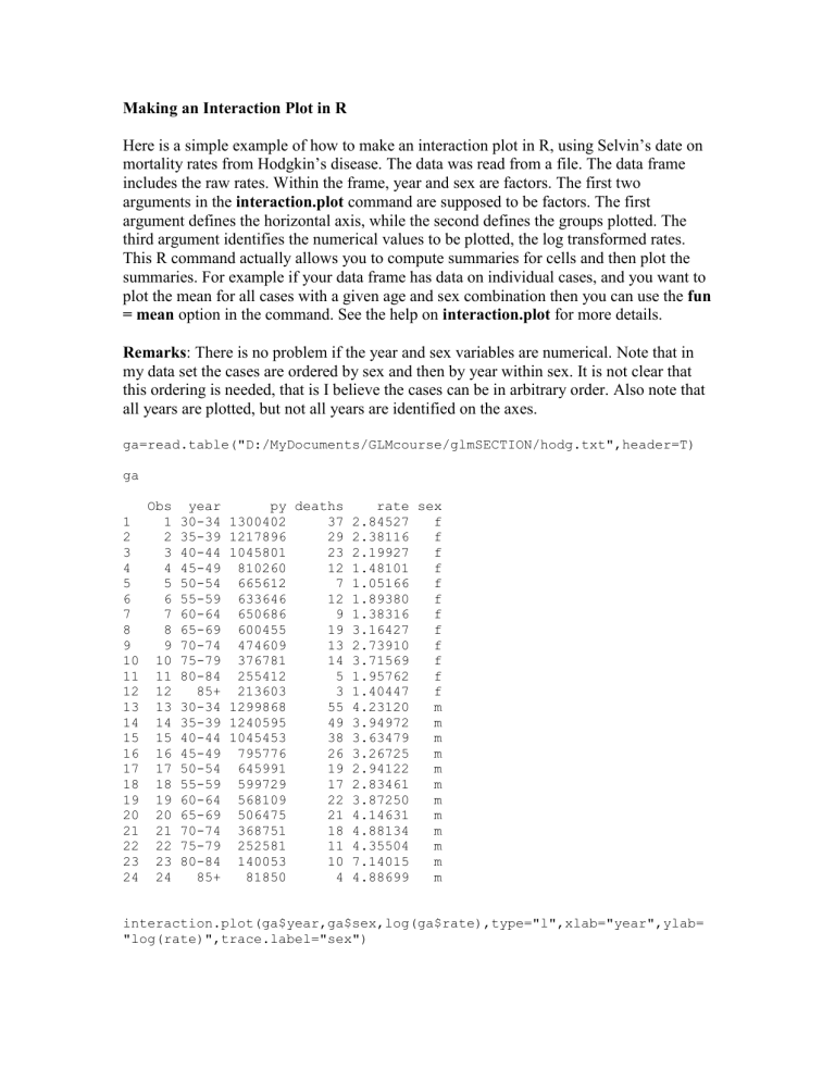
Here is a simple example of how to make an interaction plot in R, using Selvin’s date on mortality rates from Hodgkin’s disease. The data was read from a file. The data frame includes the raw rates. Within the frame, year and sex are factors. The first two arguments in the interaction.plot command are supposed to be factors. The first argument defines the horizontal axis, while the second defines the groups plotted. The third argument identifies the numerical values to be plotted, the log transformed rates.
This R command actually allows you to compute summaries for cells and then plot the summaries. For example if your data frame has data on individual cases, and you want to plot the mean for all cases with a given age and sex combination then you can use the fun
= mean option in the command. See the help on interaction.plot
for more details.
Remarks : There is no problem if the year and sex variables are numerical. Note that in my data set the cases are ordered by sex and then by year within sex. It is not clear that this ordering is needed, that is I believe the cases can be in arbitrary order. Also note that all years are plotted, but not all years are identified on the axes. ga=read.table("D:/MyDocuments/GLMcourse/glmSECTION/hodg.txt",header=T) ga
Obs year py deaths rate sex
1 1 30-34 1300402 37 2.84527 f
2 2 35-39 1217896 29 2.38116 f
3 3 40-44 1045801 23 2.19927 f
4 4 45-49 810260 12 1.48101 f
5 5 50-54 665612 7 1.05166 f
6 6 55-59 633646 12 1.89380 f
7 7 60-64 650686 9 1.38316 f
8 8 65-69 600455 19 3.16427 f
9 9 70-74 474609 13 2.73910 f
10 10 75-79 376781 14 3.71569 f
11 11 80-84 255412 5 1.95762 f
12 12 85+ 213603 3 1.40447 f
13 13 30-34 1299868 55 4.23120 m
14 14 35-39 1240595 49 3.94972 m
15 15 40-44 1045453 38 3.63479 m
16 16 45-49 795776 26 3.26725 m
17 17 50-54 645991 19 2.94122 m
18 18 55-59 599729 17 2.83461 m
19 19 60-64 568109 22 3.87250 m
20 20 65-69 506475 21 4.14631 m
21 21 70-74 368751 18 4.88134 m
22 22 75-79 252581 11 4.35504 m
23 23 80-84 140053 10 7.14015 m
24 24 85+ 81850 4 4.88699 m interaction.plot(ga$year,ga$sex,log(ga$rate),type="l",xlab="year",ylab=
"log(rate)",trace.label="sex")

sex f m
30-34 40-44 50-54 60-64 year
70-74 80-84