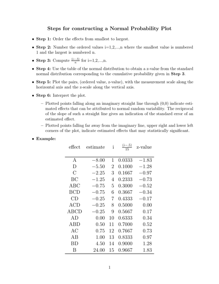
Steps for constructing a Normal Probability Plot
• Step 1: Order the effects from smallest to largest.
• Step 2: Number the ordered values i=1,2,...,n where the smallest value is numbered
1 and the largest is numbered n.
• Step 3: Compute
(i−.5)
n
for i=1,2,...,n.
• Step 4: Use the table of the normal distribution to obtain a z-value from the standard
normal distribution corresponding to the cumulative probability given in Step 3.
• Step 5: Plot the pairs, (ordered value, z-value), with the measurement scale along the
horizontal axis and the z-scale along the vertical axis.
• Step 6: Interpret the plot.
– Plotted points falling along an imaginary straight line through (0,0) indicate estimated effects that can be attributed to normal random variability. The reciprocal
of the slope of such a straight line gives an indication of the standard error of an
estimated effect.
– Plotted points falling far away from the imaginary line, upper right and lower left
corners of the plot, indicate estimated effects that may statistically significant.
• Example:
effect
A
D
C
BC
ABC
BCD
CD
ACD
ABCD
AD
ABD
AC
AB
BD
B
estimate
i
(i−.5)
15
z-value
−8.00
−5.50
−2.25
−1.25
−0.75
−0.75
−0.25
−0.25
−0.25
0.00
0.50
0.75
1.00
4.50
24.00
1
2
3
4
5
6
7
8
9
10
11
12
13
14
15
0.0333
0.1000
0.1667
0.2333
0.3000
0.3667
0.4333
0.5000
0.5667
0.6333
0.7000
0.7667
0.8333
0.9000
0.9667
−1.83
−1.28
−0.97
−0.73
−0.52
−0.34
−0.17
0.00
0.17
0.34
0.52
0.73
0.97
1.28
1.83
1