PARAMETRICAL REGULATION OF ECONOMIC GROWTH BASED ON THE
TURNOVSKY MONETARY MODEL
Abdykappar A. Ashimov, Bahyt T. Sultanov, Zheksenbek M. Adilov, Yuriy V. Borovskiy, Dauren K. Suissinbayev,
Askar A. Ashimov
Kazakh National Technical University
050013, Almaty, 22 Satpayev Str, Republic of Kazakhstan
Email: ashimov37@mail.ru, yuborovskiy@gmail.com, daurensmail@gmail.com
ABSTRACT
The work presents the application results of the
parametrical regulation theory in the sphere of economic
growth based on the Turnovsky monetary model. We
present the results of the solution to the problem of
parametrical identification of the considered model. The
evaluation of a weak structural stability of the Turnovsky
model in the compact domain of the phase space was
obtained. Optimal (in sense of the criterion characterizing
an economic growth) values of regulated parameters of
the model and the dependence of a criterion’s optimal
values on the two unregulated parameters were found.
KEY WORDS
Оptimal control, nonlinear systems, modelling and
simulation, parametrical regulation.
1. Introduction
The national economy interacting with economic systems
of other different countries is quite a difficult object to
manage. Today the issues of government regulation of the
national economy evolution (economic growth) are
considered on the basis of macroeconomic mathematical
models, basically applying the scenario approach. During
the scenario approach to the development of national
economic policy on the basis of the selected model, the
scenario variants are iterated applying different sets of
economic tools (parameters regulated by the government)
and applying the analysis of the obtained corresponding
solutions of the examined model [10, 11]. Thus in the
known literature and practice there are no scientific
propositions of parametrical regulation of market
economy development that meets the requirements of
optimality of the state’s economic system evolution and
the recommendations for the development and
implementation of effective state economic policy.
A lot of dynamic systems, including the country's
economic system, after some transformations can be
represented by systems of nonlinear ordinary differential
equations containing in its right-hand side vectors of
regulated (controlled) (𝑢) parameters and vectors of
unregulated parameters(disturbances) (λ) as well.
As it is known, the solution (evolution) of the
examined system of the differential equations depends on
the vector of initial values of the system and on the values
of 𝑢 and λ vectors as well. Therefore, the result of
evolution (development) of a nonlinear dynamic system
with a given vector of initial values is determined by the
values of vectors of both regulated and unregulated
parameters.
Also it is known [8] that we can judge by the solution
of the dynamic systems about the object it describes, if the
system has the property of immutability of the qualitative
picture of the trajectory, when there are small in some
sense perturbations of the right side of the system. In
other words, a dynamic system must be robust, or
structurally stable.
Based on the aforesaid, in [2] – [5] we propose a
theory of parametrical regulation of market economy
development (the effectiveness of which is shown on a
number of applications). This paper examines the
application of the theory of parametrical regulation to
estimate the optimal values of parameters (tools) of public
policy in the sphere of economic growth based on the
Turnovsky monetary model.
2. Model description
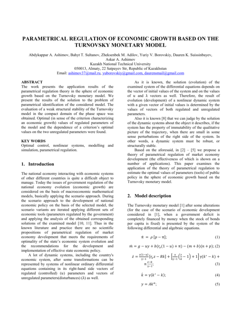
The Turnovsky monetary model [1] after some alterations
(for the case of the scenario of economic development
considered in [1], when a government deficit is
completely financed by money when the stock of bonds
per capita is fixed) is presented by the system of the
following differential and algebraic equations.
π̇ = 𝜌 [𝑝 − π];
(1)
𝑚̇ = 𝑔 − 𝑢𝑦 + 𝑏(𝑟𝑒 (1 − 𝑢) + π) − (𝑚 + 𝑏)(𝑛 + 𝑝); (2)
𝑧̇ =
γ(1−𝑢)
γ−1
𝑛
[𝑟𝑒 𝑧 − 𝑅𝑘] + [
γ
𝑧
( − 1) + 1] γ(𝑘 ∗ − 𝑘) +
γ−1 𝑘
𝑧−𝑘
;
(3)
𝑘̇ = γ(𝑘 ∗ − 𝑘);
(4)
𝑦 = 𝐴𝑘 α ;
(5)
γ−1
𝑟𝑒 = 𝐴α𝑘 ∗ α−1 ;
(6)
𝑅 = 𝐴α𝑘 α−1 ;
(7)
𝑘∗ =
𝑦−𝑐[(𝑦−𝑅𝑘)(1−𝑢)+
𝑏+𝑧
[(1−𝑙4 )𝑚−𝑙4 (𝑏+𝑧)−𝑙1 𝑦+𝑙3 𝜋]+𝑧𝑛−𝑚𝜋]−𝑛𝑘+𝑔
𝑙2
𝑐𝑧
λ[ −𝑐+1]
𝑘
;
(8)
𝑖 = λ(𝑘 ∗ − 𝑘) + 𝑛𝑘.
(9)
Here dot denotes the derivative with respect to time (t),
measured in years.
Output (endogenous) variables of the model:
π – instantaneous expected rate of inflation (1/year);
𝑚 – nominal per capita stock of outside money
(tenge/person), tenge - national currency of Kazakhstan;
𝑧 – real per capita volume of shares (tenge/person),
(real indices here and in further are determined by the
prices of the year of 2000);
𝑘 – real capital-labor ratio (tenge/person);
𝑦 – real per capita output (tenge/(person*year));
𝑟𝑒 – real before-tax rate of return on securities
(1/year);
𝑅 – marginal real physical product of capital
(tenge/(person*year2));
𝑘 ∗ – desires real per capita stock of capital
(tenge/person);
𝑖 – real per capita investments (tenge/(person*year));
Input (exogenous) time dependent variables of the
model:
𝑝 – consumer price index (1/year);
𝑔 – real per capita government spending
(tenge/(person*year)) (𝑔 > 0);
𝑛 – rate of growth of population (1/year);
γ – coefficient of the capital-labor ratio (1/year) (0 <
𝛾 < 1);
𝐴, α – coefficients of production function (𝐴 > 0,
0 < 𝛼 < 1);
𝑐 – share of real per capita consumption out of real
disposable income (0 < 𝛼 < 1) (dimensionless);
𝑙1 , 𝑙2 , 𝑙3 , 𝑙4 – coefficients of real per capita demand
for money equations (𝑙1 > 0, 𝑙2 < 0, 𝑙3 > 0, 0 < 𝑙4 < 1)
(dimensionless);
λ – coefficient of per capita investment rate, λ > 0
(1/year);
𝑢 – income tax rate, 0 < 𝑢 < 1 (dimensionless);
Input parameters of the model:
𝑏 – nominal per capita stock of government; 𝑏 > 0
(tenge/person).
Input parameters of the model involve initial values
(when 𝑡 = 0) of output variables of the dynamic
equations of the model (1) – (4): π0 , 𝑚0 , 𝑧0 , 𝑘0 . The
values of input functions of the model at integer 𝑡 time
values are also considered as input parameters of the
model. All input functions of the model are considered as
sectionally linear continuous functions that
determined by their values for integral values of 𝑡.
are
3. Evaluation of the Turnovsky model’s
parameters
and
a
retrospective
forecasting
As a part of the solution to the problem of evaluation of
the model’ input parameters (parametrical identification)
we obtained the values of the following input functions
and parameters 𝑝(𝑡), 𝑔(𝑡), 𝑛(𝑡), γ(𝑡), 𝐴(𝑡), α(𝑡), λ(𝑡),
𝑐(𝑡), 𝑙1 (𝑡), 𝑙2 (𝑡), 𝑙3 (𝑡), 𝑙4 (𝑡), 𝑢(𝑡) where 𝑡 = 0, 1, … , 9,
and 𝑏, π0 , 𝑚0 , 𝑧0 , 𝑘0 applying the searching method in
sense of the criterion minimum (the sum of the squares of
the residuals of the output variables) based on statistical
data of the Republic of Kazakhstan economy evolution
for 2000 – 2009. The values of the input functions and
parameters were sought in the small intervals centered at
the observed values of the corresponding functions and
parameters (in case of their presence).
The criterion of the parametrical identification has the
following type (10).
𝐾𝐼 = ∑ν
1
𝑛
𝑗=1 ∑𝑡=0 𝑀𝑗𝑡
𝑥𝑗 (𝑡)−𝑥𝑗∗ (𝑡)
∑ν𝑗=1 ∑𝑛𝑡=0 𝑀𝑗𝑡 (
𝑥𝑗∗ (𝑡)
2
) → min.
(10)
Here ν = 5 – the number of output variables, used in the
evaluation of the parameters, 𝑗 – number of the variable;
𝑛 + 1 – number of observations, 𝑡 = 0 corresponds to the
beginning of the year of 2000; 𝑥𝑗 (𝑡) – calculated values of
output variables (𝑦(𝑡), 𝑘(𝑡), 𝑧(𝑡), π(𝑡), 𝑖(𝑡)) at
corresponding time values. The sign “*” corresponds to
the observed values of the corresponding variables. 𝑀𝑗𝑡 –
positive weight coefficients, whose values were chosen on
the basis of the significance of the values of related output
variables in solving the problem of parametrical
identification of the model. Table 1 presents weights of
the criterion 𝐾𝐼 ; 𝑀𝑗𝑡 value is at the intersection of 𝑗 row
and 𝑡 column.
The Runge-Kutta and the Nelder-Mead algorithms
[7] were applied while solving the parameter evaluation
problem (𝑛 = 7). The stated problem of parametrical
identification was solved using the statistical data for the
period of 2000 – 2007. As the result of the solution to the
stated problem, the relative value of the weight average
quadratic deviation of the calculated values of the model’s
output variables from the corresponding observed values
(100√𝐾𝐼 ) did not exceed 1.2 %.
As part of the model verification the following
problem of retroforecasting was solved. Get an estimate
of relative errors of calculated values of the model’s
output variables relative to the corresponding observed
values on the interval from 2008 to 2009, applying the
obtained values of input functions, parameters, and initial
Table 1
𝑀𝑗𝑡 weigh of 𝐾𝐼 criterion
Year
2000,
𝑡=0
Variable
2001,
𝑡=1
2002,
𝑡=2
2003,
𝑡=3
2004,
𝑡=4
2005,
𝑡=5
2006,
𝑡=6
2007,
𝑡=7
𝑦(𝑡), 𝑗 = 1
0.001
0.001
0.001
0.01
0.01
1
1
1
𝑘(𝑡), 𝑗 = 2
0.001
0.001
0.001
0.001
0.001
0.001
0.001
0.001
𝑧(𝑡), 𝑗 = 3
0.001
0.001
0.001
0.01
0.01
1
1
1
𝜋(𝑡), 𝑗 = 4
0.001
0.001
0.001
0.01
0.01
0.1
0.1
0.1
𝑖(𝑡), 𝑗 = 5
0.001
0.001
0.001
0.01
0.01
0.1
0.1
0.1
values of output variables for the period 2000 – 2007
(also applying extrapolation of values of input functions
for the period of 2008 – 2009). Results of the solution to
this problem are presented in the following table (Table
2). Here sign “*” corresponds to the observed values; the
sign “Δ” corresponds to the deviations (in percentage) of
calculated values from the corresponding observed values.
For the period of retroforecasting the average error of
the variables, shown in the table, is 3.7825%, indicating
acceptable accuracy in describing the evolution of
Kazakhstan's economy with the help of the model.
Table 2
Observed, calculated values of output variables of the
model and corresponding deviations (in percentage)
Year
2008
2009
∗
336140
334680
𝑦
333843
333015
∆𝑦
𝑦
0.68322
0.49744
∗
1117488
1305937
𝑧
1228469
1483599
∆𝑧
𝑧
9.93126
13.60410
∗
747806
771832
𝑘
675539
762518
∆𝑘
9.66383
1.20669
∗
0.11828
0.07525
𝜋
0.11881
0.07639
∆𝜋
0.45321
1.51652
∗
136501
151534
𝑖
136424
151855
∆𝑖
0.05666
0.21187
𝑘
𝜋
𝑖
4. Investigation of the structural stability of
the Turnovsky monetary model
This study was conducted based on the following
Robinson [6] theorem (Theorem A) about sufficient
conditions for weak structural stability.
Suppose 𝑁′ – is some manifold, N – is a compact
subset in 𝑁′ such that the closure of 𝑀 interior is 𝑀. Let
some vector field be defined in a neighborhood of the set
𝑁 in 𝑁′, this field defines 𝐶 1 -flow 𝑓 in this neighborhood.
Let 𝑅(𝑓, 𝑀) be chain-recurrent set of flow 𝑓 on 𝑁.
Let 𝑅(𝑓, 𝑁) be contained inside of 𝑁. Let it have
hyperbolic structure, additionally flow 𝑓 on 𝑅(𝑓, 𝑁) also
satisfies the transversality conditions of stable and
unstable manifolds. Then flow 𝑓 on 𝑁 is weakly
structurally stable. In particular, if 𝑅(𝑓, 𝑁) is the empty
set, then the 𝑓 flow is weakly structurally stable on 𝑁.
The analogous result is true for a discrete dynamic system
(a cascade), defined by the homeomorphism (with image)
𝑓: 𝑁′ → 𝑁.
Below, based on the algorithm for constructing the
symbolic image [9] we propose the algorithm for the
localization of the chain-recurrent set for a compact subset
of phase space of a dynamical system described by a
system of ordinary differential and algebraic equations.
For computer simulation of the chain-recurrent set we
used an oriented graph (a symbolic image), which is a
discretization of the mapping shift along the trajectories
determined by this dynamic system. For a specific
mathematical model of economic system we can take as a
compact 𝑁, for example, a parallelepiped from its phase
space, which includes all the possible trajectories of
economic system evolution for the examined period of
time.
Description of the algorithm for localization of a
chain-recurrent set consists of the following.
1. The mapping 𝑓 is set, defined in 𝑁 and by a shift
along the trajectories of a dynamical system for a fixed
period of time.
2. 𝐶 partition of the compact 𝑁 into 𝑁𝑖 cells is
constructed. The oriented graph 𝐺 is specified whose
nodes correspond to cells, and edges connecting 𝑁𝑖 cells
with 𝑁𝑗 correspond to the conditions of intersection of the
image of one cell 𝑓(𝑁𝑖 ) with another cell 𝑁𝑗 .
3. The graph 𝐺 contains all returning nodes (nodes
belonging to cycles). If the set of such nodes is empty,
then 𝑅(𝑓, 𝑁) is empty and the process of its localization is
complited. The conclusion about a weak structural
stability of a dynamical systems is made.
4. Cells related to returning nodes of the graph 𝐺 are
divided into smaller cells, and the oriented graph 𝐺 is
constructed according to them (See step 2 of the
algorithm).
5. Transition to the step 3.
Steps 3, 4, 5 are repeated until the diameters of the
cells of the partition will not be less than some
preassigned number ε.
The last set of cells is evaluation of the chainrecurrent set 𝑅(𝑓, 𝑁).
The research of structural stability of the model (1) –
(9) was conducted based on: the theorem about sufficient
conditions of weak structural stability, by localization of
the chain-recurrent set 𝑅(𝑓, 𝑁) based on the algorithm
and under the additional assumption of constancy of all
input functions of the model. In this case the equations (1)
– (9) determine the flow 𝑓 in the four-dimensional phase
space of the model’s output variables (π, 𝑚, 𝑧, 𝑘).
In the presented algorithm 𝑓 mapping was
determined as a shift along the trajectories of the dynamic
system (1) – (9) that corresponds to the change of time 𝑡
by 1 (year). Input functions of the model were defined as
constant (their values for 2007 were taken).
During the application of the given above algorithm
we used the parallelepiped {0 ≤ π ≤ 0.2, 0 ≤ 𝑚 ≤ 8000,
0 ≤ 𝑧 ≤ 50000, 0 ≤ 𝑘 ≤ 830000} in the phase space of
the model (1) – (9) as the initial compact 𝑁. Partition of
the initial parallelepiped (and of the other cells, obtained
as a result of the algorithm application) into 16 parts was
done by dividing of its all edges into two equal parts. As a
result of the calculation of the developed programme after
4 iterations that were run in accordance with the given
above algorithm, we obtained the graph 𝐺 with empty sets
of nodes.
This means that the investigated Turnovsky monetary
model with considered values of input parameters is
assessed as weakly structurally stable in the specified
compact 𝑁.
5. Evaluation of the Turnovsky model’s
parametrical sensitivity
coefficients of the stated output values of the model
relative to its input values, calculated using the formula:
𝐹𝑝𝑗 (𝑡) = 100
𝑥𝑗 (𝑡)
.
(11)
Here 𝑝 – variable input parameter or the value of input
function; 𝑥𝑗 (𝑡) – value of 𝑗-th output variable for 𝑡 time
obtained when running the model with values of input
parameters and functions, obtained as a result of the
parameter evaluation or taken from statistical sources (the
basic calculation); 𝑥𝑗𝑛 (𝑡) – value of the corresponding
output variable, obtained when increasing the value of the
input variable parameter 𝑝 by 1%, while the remaining
values of input parameters and functions remain
unchanged compared to the basic calculation.
The results of solving the problem by constructing a
matrix of parametrical sensitivity are partially shown in
Table 3. For example, when the value of the parameter
𝑐(9) increases by 1% and when the value of 𝑐(8) remains
unchanged, the linear function 𝑐(𝑡) correspondingly
increases in the interval [8], [9], this in its turn involves
the change in values of output variables (and coefficients
𝐹𝑝𝑗 (𝑡)) when 𝑡 = 9.
The analysis of Table 3 indicates, that within the
given input parameters for the year of 2009, the output
variables 𝑦(9), 𝑚(9), 𝑧(9), 𝑘(9), 𝑖(9) are mostly
affected by the change in the coefficient of the production
function α(9), and the output variable π(9) can only be
affected by the change of price index 𝑝(9).
6. Finding optimal values of regulated
parameters based on the Turnovsky
model
We now consider the possibility of implementing an
effective government policy based on the model (1) – (9)
through the synthesis of optimal values of economic
parameters: per capita government spending 𝑔(𝑡) and the
income tax rate 𝑢(𝑡) for the period 2010 – 2015. The
synthesis problem of an optimal law of parametrical
regulation on the level of mentioned parameters 𝑔(𝑡) and
𝑢(𝑡) can be formulated in the following way. Based on
the mathematical model (1) – (9) find such values of
𝑔(𝑡), 𝑢(𝑡), 𝑡 = 10, … ,15, that would provide the
maximum of the criterion (average of real per capita
output for the period 2010 – 2015)
1
As part of the solution to the problem of assessing the
impact of the values of input parameters and functions of
the model on the values of its output variables we
constructed a matrix whose rows are indexed by all the
input parameters and functions, and columns – by the
values of the six output variables for 𝑡 = 9, which
corresponds to 2009. This matrix contains the sensitivity
𝑥𝑗𝑛(𝑡)−𝑥𝑗 (𝑡)
𝐾 = ∑15
𝑡=10 𝑦(𝑡)
6
(12)
under the following constrains imposed on the model’s
output variables and regulated parameters (here 𝑡 ∈
[10, 15]).
Table 3
Some elements of the parametrical sensitivity of the model for 𝑡 = 9
Output variable
𝑧(9)
𝑘(9)
𝑐(9)
-0.01637
𝑦(9)
0
-0.0123
0.00309
-0.0165
1.693064
𝑔(9)
0.280699
0
0.26993
0.33196
0.28325
0.881013
𝑛(9)
-0.01726
0
-0.0206
-0.0293
-0.0174
0.048407
𝑝(9)
-0.00993
0.5161
-0.052
-0.0136
-0.01
-0.3979
λ(9)
-0.03802
0
0.0294
-0.0888
-0.0384
-2.59267
γ(9)
0.136572
0
-0.002
-0.2708
0.13781
-0.45509
𝐴(9)
0.790219
0
-0.0334
-0.2985
-0.2096
-3.41885
α(9)
11.38849
0
-0.3144
-2.2215
-2.6097
-53.2406
Input Parameter
π(9)
𝑚(9)
𝑖(9)
𝑙1 (9)
-0.16371
0
0.0578
-0.2697
-0.1652
-4.8311
𝑙2 (9)
0.009145
0
0.01151
-0.0083
0.00923
-1.51853
𝑙3 (9)
-0.04331
0
-0.0052
-0.0387
-0.0437
0.849691
𝑙4 (9)
-0.14034
0
0.0436
-0.2246
-0.1416
-3.58984
π(𝑡) > 0, 𝑚(𝑡) > 0, 𝑧(𝑡) > 0, 𝑘(𝑡) > 0,
𝑘 ∗ (𝑡) > 0, 𝑖(𝑡) > 0,
𝑔(𝑡) > 0, 0 < 𝑢(𝑡) < 1.
(13)
(14)
Note that for the basic calculation of the model for
the period till 2015, that was obtained at determined
values of the model’s input parameters and with the help
of extrapolation of the model’s input functions by linear
trend, the value of the criterion turned out to be 𝐾 =
437368 tenge (in prices of the year 2000).
As the result of the numerical solution to the stated
problem of finding optimal values of 𝑔(𝑡), 𝑢(𝑡)
parameters of economic system applying the NelderMead algorithm [7] we obtained the optimal result 𝐾 =
511552. Compared to the basic variant, if to apply the
considered above parametrical regulation, the increase in
the value of 𝐾 criterion was 16.96%.
Graphs of calculated values of the model’s output
variable – real per capita output (𝑦(𝑡)) without
parametrical regulation, and applying the found optimal
law of parametrical regulation, are presented below in
Figure 1.
Figure 1. Real per capita output
7. Investigation of the dependence of the
optimal values of the parametrical
regulation criterion on the values of
unregulated parameters based on the
Turnovsky model
The considered above optimization problem was solved at
fixed values of input parameters that are not involved in
the regulation. In addition, during the research we found
the dependence of optimal values of the criterion 𝐾 on the
values of unregulated parameters of the model by the
example of two-dimensional parameter 𝑎 = (𝑐(9), λ(9))
consisting of a share of real consumption out of real
disposable income and the investment coefficient for
2009. The range of variation of these parameters was
determined based on the estimated values of 𝑐(9) and
λ(9) in the form of the rectangle 𝐴 = [0.0820; 0.1090] ×
[0.708; 0.719].
Figure 2 shows some results of studies: graphs of the
dependence of 𝐾 criterion on 𝑎 parameter (where 𝑎 ∈ 𝐴)
for the considered above problem of parametrical
regulation. Graphs in Figure 2 describe the basic and
optimal (for the problem of finding per capita government
spending and income tax rates) values of the criterion 𝐾.
Figure 2.
– basic variant,
– regulation of per capita
government spending and income tax rates
8. Conclusion
1. The results of solving the problem of parametrical
identification of the considered model are presented.
2. The estimate of the weak structural stability of the
Turnovsky model in a compact domain of the phase space
was obtained.
3. The optimal (in the sense of characterizing
economic growth) the values of regulated parameters of
the model were found.
4. The dependence of the optimal values of the
criterion that characterizes an economic growth on the
two uncontrolled parameters was found.
The obtained results can be used in the development
and implementation of an effective state policy.
References
[1] S. Turnovsky. Macroeconomic Dynamics and Growth
in a Monetary Economy: a Synthesis, Journal of money,
Credit and Banking, 10(Issue 1), 1978, 1-26.
[2] A.A. Ashimov, B.T. Sultanov, Zh.M. Adilov, Yu.V.
Borovskiy, D.A. Novikov, R.M. Nizhegorodcev, & As.A.
Ashimov, Macroeconomic analysis and economic policy
based on parametrical regulation (Moscow: Physmatlit,
2010, in Russian).
[3] А.А. Ashimov, N.A. Iskakov, Yu.V. Borovskiy, B.T.
Sultanov, & As.А. Ashimov, Parametrical regulation of
economic growth on the basis of one-class mathematical
models, Systems Science, 35(1), 2009, 57-63.
[4] A.A. Ashimov, K.A. Sagadiyev, Yu.V. Borovskiy,
N.A. Iskakov, & Аs.A. Ashimov, Elements of the market
economy development parametrical regulation theory,
Proc. 9th IASTED International Conf. on Control and
Application, Montreal, Quebec, Canada, 2007, 296-301.
[5] A.A. Ashimov, K.A. Sagadiyev, Yu.V. Borovskiy,
N.A. Iskakov, As.A. Ashimov, On the market economy
development parametrical regulation theory, Kybernetes,
The international journal of cybernetics, systems and
management sciences, 37(5), 2008, 623-636.
[6] C. Robinson, Structural Stability on Manifolds with
Boundary, Journal of differential equations, (37), 1980, 111.
[7] J.A Nelder & R. Mead, A simplex method for function
minimization, The Computer Journal, (7), 1965, 308-313.
[8] V.I. Arnold, Geometrical Methods in the Theory of
Ordinary Differential Equations (Berlin: Springer-Verlag,
1997).
[9] E.I. Petrenko, Development and Implementation of
Algorithms for Construction of the Symbolic Image,
Electronic journal “Differential equations and control
processes”, (3), 2006, 55-96.
[10] V.L Makarov, A.R Bahtizin, & S.S. Sulakshin,
Application of computable models in state administration.
(Moscow: Scientific expert, 2007, in Russian).
[11] S.J. Turnovsky, Methods of Macroeconomic
Dynamics, (Cambridge: MIT Press, 2000).