Problem Statement
Last year, five randomly selected students took a math aptitude test before they began their
statistics course. The Statistics Department has three questions.



What linear regression equation best predicts statistics performance, based on math
aptitude scores?
If a student made an 80 on the aptitude test, what grade would we expect her to make in
statistics?
How well does the regression equation fit the data?
How to Find the Regression Equation
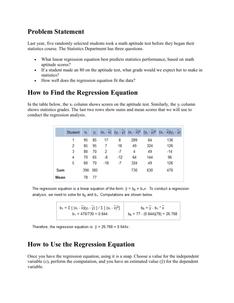
In the table below, the xi column shows scores on the aptitude test. Similarly, the yi column
shows statistics grades. The last two rows show sums and mean scores that we will use to
conduct the regression analysis.
How to Use the Regression Equation
Once you have the regression equation, using it is a snap. Choose a value for the independent
variable (x), perform the computation, and you have an estimated value (ŷ) for the dependent
variable.
In our example, the independent variable is the student's score on the aptitude test. The
dependent variable is the student's statistics grade. If a student made an 80 on the aptitude test,
the estimated statistics grade would be:
ŷ = 26.768 + 0.644x = 26.768 + 0.644 * 80 = 26.768 + 51.52 = 78.288
Warning: When you use a regression equation, do not use values for the independent variable
that are outside the range of values used to create the equation. That is called extrapolation, and
it can produce unreasonable estimates.
In this example, the aptitude test scores used to create the regression equation ranged from 60 to
95. Therefore, only use values inside that range to estimate statistics grades. Using values outside
that range (less than 60 or greater than 95) is problematic
How to Find the Coefficient of Determination
Whenever you use a regression equation, you should ask how well the equation fits the data. One
way to assess fit is to check the Coefficient of Determination
The coefficient of determination (denoted by R2) is a key output of regression analysis. It is
interpreted as the proportion of the variance in the dependent variable that is predictable from the
independent variable.





The coefficient of determination is the square of the correlation (r) between predicted y
scores and actual y scores; thus, it ranges from 0 to 1.
With linear regression (the type of regression we are using in this tutorial), the coefficient
of determination is also equal to the square of the correlation between x and y scores.
An R2 of 0 means that the dependent variable cannot be predicted from the independent
variable.
An R2 of 1 means the dependent variable can be predicted without error from the
independent variable.
An R2 between 0 and 1 indicates the extent to which the dependent variable is
predictable. An R2 of 0.10 means that 10 percent of the variance in Y is predictable from
X; an R2 of 0.20 means that 20 percent is predictable; and so on.
The formula for computing the coefficient of determination for a linear regression model with
one independent variable is given below.
Coefficient of determination. The coefficient of determination (R2) for a linear regression
model with one independent variable is:
R2 = { ( 1 / N ) * Σ [ (xi - x) * (yi - y) ] / (σx * σy ) }2
where N is the number of observations used to fit the model, Σ is the summation symbol, xi is the
x value for observation i, x is the mean x value, yi is the y value for observation i, y is the mean y
value, σx is the standard deviation of x, and σy is the standard deviation of y. Computations for
the sample problem of this lesson are shown below.
σx = sqrt [ Σ ( xi - x )2 / N ]
σx = sqrt( 730/5 ) = sqrt(146) = 12.083
σy = sqrt [ Σ ( yi - y )2 / N ]
σy = sqrt( 630/5 ) = sqrt(126) = 11.225
R2 = { ( 1 / N ) * Σ [ (xi - x) * (yi - y) ] / (σx * σy ) }2
R2 = [ ( 1/5 ) * 470 / ( 12.083 * 11.225 ) ]2 = ( 94 / 135.632 )2 = ( 0.693 )2 = 0.48
A coefficient of determination equal to 0.48 indicates that about 48% of the variation in statistics grades
(the dependent variable) can be explained by the relationship to math aptitude scores (the independent
variable).
Residual Plots
A residual plot is a graph that shows the residuals on the vertical axis and the independent
variable on the horizontal axis. If the points in a residual plot are randomly dispersed around the
horizontal axis, a linear regression model is appropriate for the data; otherwise, a non-linear
model is more appropriate.
Below the table on the left shows inputs and outputs from a simple linear regression analysis,
and the chart on the right displays the residual (e) and independent variable (X) as a residual plot.
x
60
70
80
85
95
y
70
65
70
95
85
ŷ
65.411
71.849
78.288
81.507
87.945
e
4.589
-6.849
-8.288
13.493
-2.945
The residual plot shows a fairly random pattern - the first residual is positive, the next two are
negative, the fourth is positive, and the last residual is negative. This random pattern indicates
that a linear model provides a decent fit to the data.
Below, the residual plots show three typical patterns. The first plot shows a random pattern,
indicating a good fit for a linear model. The other plot patterns are non-random (U-shaped and
inverted U), suggesting a better fit for a non-linear model.
Random pattern
Non-random: U-shaped
Non-random: Inverted U
Which of the following statements are true?
I. When the sum of the residuals is greater than zero, the data set is nonlinear.
II. A random pattern of residuals supports a linear model.
III. A random pattern of residuals supports a non-linear model.
(A) I only
(B) II only
(C) III only
(D) I and II
(E) I and III
Solution
The correct answer is (B). A random pattern of residuals supports a linear model; a non-random
pattern supports a non-linear model. The sum of the residuals is always zero, whether the data set
is linear or nonlinear.
Influential Points
An influential point is an outlier that greatly affects the slope of the regression line. One way to
test the influence of an outlier is to compute the regression equation with and without the outlier.
Which of the following statements are true?
I. When the data set includes an influential point, the data set is nonlinear.
II. Influential points always reduce the coefficient of determination.
III. All outliers are influential data points.
(A) I only
(B) II only
(C) III only
(D) All of the above
(E) None of the above
Solution
The correct answer is (E). Data sets with influential points can be linear or nonlinear