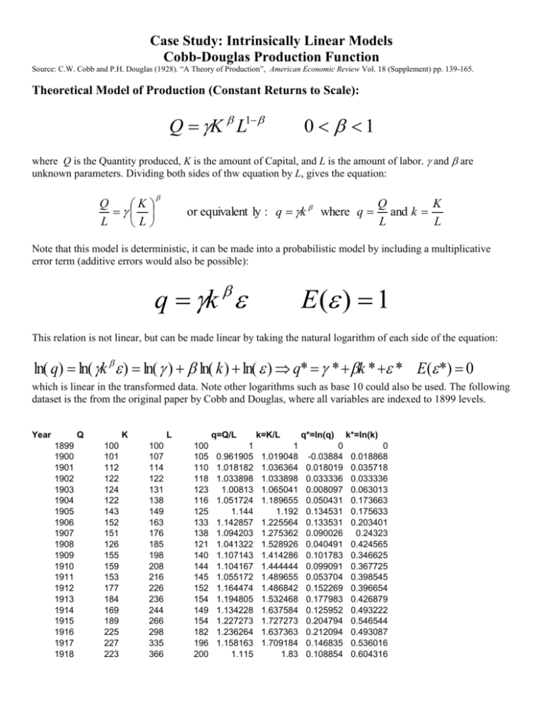
Case Study: Intrinsically Linear Models
Cobb-Douglas Production Function
Source: C.W. Cobb and P.H. Douglas (1928). “A Theory of Production”, American Economic Review Vol. 18 (Supplement) pp. 139-165.
Theoretical Model of Production (Constant Returns to Scale):
Q  K  L1 
0   1
where Q is the Quantity produced, K is the amount of Capital, and L is the amount of labor.  and  are
unknown parameters. Dividing both sides of thw equation by L, gives the equation:
Q
K
 
L
L

or equivalent ly : q  k  where q 
Q
K
and k 
L
L
Note that this model is deterministic, it can be made into a probabilistic model by including a multiplicative
error term (additive errors would also be possible):
q  k  
E ( )  1
This relation is not linear, but can be made linear by taking the natural logarithm of each side of the equation:
ln( q)  ln( k   )  ln(  )   ln( k )  ln(  )  q*   *  k *  * E ( *)  0
which is linear in the transformed data. Note other logarithms such as base 10 could also be used. The following
dataset is the from the original paper by Cobb and Douglas, where all variables are indexed to 1899 levels.
Year
Q
1899
1900
1901
1902
1903
1904
1905
1906
1907
1908
1909
1910
1911
1912
1913
1914
1915
1916
1917
1918
K
100
101
112
122
124
122
143
152
151
126
155
159
153
177
184
169
189
225
227
223
L
100
107
114
122
131
138
149
163
176
185
198
208
216
226
236
244
266
298
335
366
q=Q/L
100
105
110
118
123
116
125
133
138
121
140
144
145
152
154
149
154
182
196
200
1
0.961905
1.018182
1.033898
1.00813
1.051724
1.144
1.142857
1.094203
1.041322
1.107143
1.104167
1.055172
1.164474
1.194805
1.134228
1.227273
1.236264
1.158163
1.115
k=K/L
1
1.019048
1.036364
1.033898
1.065041
1.189655
1.192
1.225564
1.275362
1.528926
1.414286
1.444444
1.489655
1.486842
1.532468
1.637584
1.727273
1.637363
1.709184
1.83
q*=ln(q)
0
-0.03884
0.018019
0.033336
0.008097
0.050431
0.134531
0.133531
0.090026
0.040491
0.101783
0.099091
0.053704
0.152269
0.177983
0.125952
0.204794
0.212094
0.146835
0.108854
k*=ln(k)
0
0.018868
0.035718
0.033336
0.063013
0.173663
0.175633
0.203401
0.24323
0.424565
0.346625
0.367725
0.398545
0.396654
0.426879
0.493222
0.546544
0.493087
0.536016
0.604316
1919
1920
1921
1922
218
231
179
240
387
407
417
431
193
193
147
161
1.129534
1.196891
1.217687
1.490683
2.005181
2.108808
2.836735
2.677019
0.121805
0.179728
0.196953
0.399235
0.695735
0.746123
1.042654
0.984704
Step 1: Fit a simple regression model, regressing q* on k*:
Intercept estimates ln(and coefficient of k* estimates :
Intercept
k*=ln(k)
Coefficient Standard
t Stat
P-value
s
Error
0.014545 0.019979 0.727985 0.474301
0.254134 0.041224 6.164776 3.32E-06
Step 2: Right out linear equation in transformed q and k:
^
q *  0.014545  0.254134k *
Step 3: Back transform the model (exponentiating both sides):
^
q  e 0.0145450.254134k *  e 0.0145e 0.254ln(k )  1.0146k 0.254
Plot of data and the function:
Q
K
 1.0146 
L
L
0.254
Regression Plot
1.6
1.5
Q/L
1.4
1.3
1.2
1.1
1
.9
.8
1
1.2
1.4 1.6 1.8 2
K/L
Y = 1.015 * (X^.254)
2.2 2.4
2.6 2.8
3