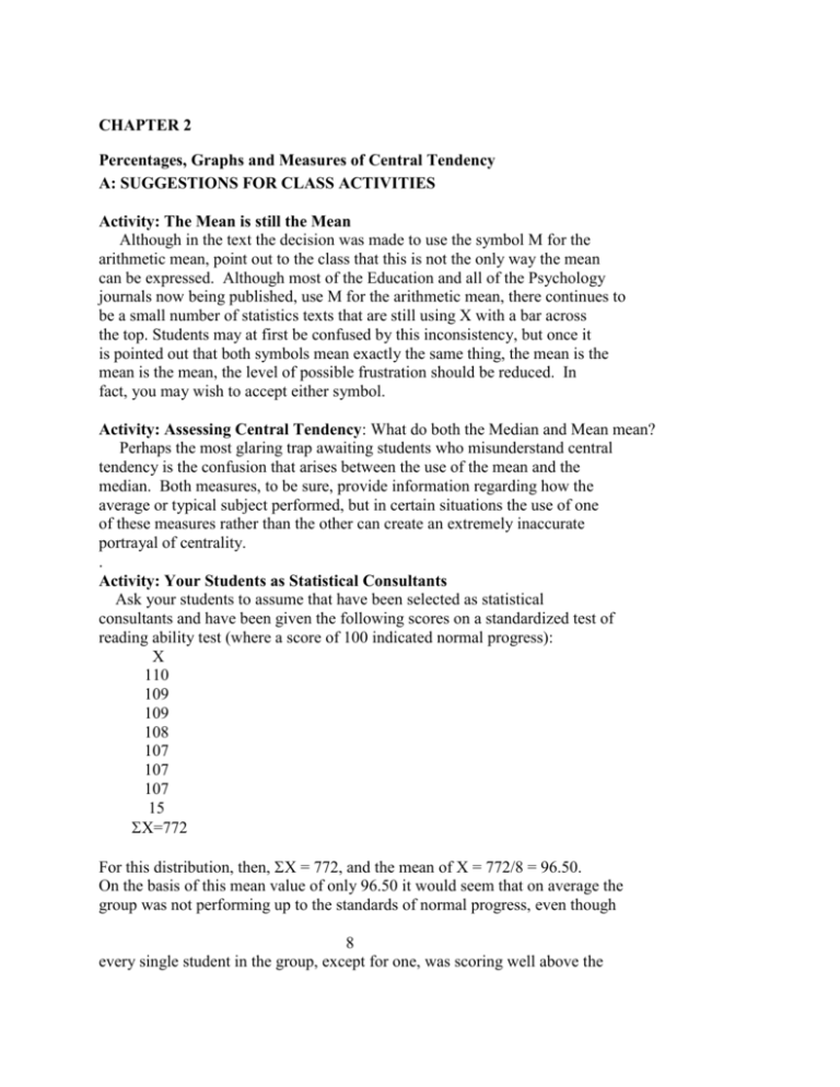
CHAPTER 2
Percentages, Graphs and Measures of Central Tendency
A: SUGGESTIONS FOR CLASS ACTIVITIES
Activity: The Mean is still the Mean
Although in the text the decision was made to use the symbol M for the
arithmetic mean, point out to the class that this is not the only way the mean
can be expressed. Although most of the Education and all of the Psychology
journals now being published, use M for the arithmetic mean, there continues to
be a small number of statistics texts that are still using X with a bar across
the top. Students may at first be confused by this inconsistency, but once it
is pointed out that both symbols mean exactly the same thing, the mean is the
mean is the mean, the level of possible frustration should be reduced. In
fact, you may wish to accept either symbol.
Activity: Assessing Central Tendency: What do both the Median and Mean mean?
Perhaps the most glaring trap awaiting students who misunderstand central
tendency is the confusion that arises between the use of the mean and the
median. Both measures, to be sure, provide information regarding how the
average or typical subject performed, but in certain situations the use of one
of these measures rather than the other can create an extremely inaccurate
portrayal of centrality.
.
Activity: Your Students as Statistical Consultants
Ask your students to assume that have been selected as statistical
consultants and have been given the following scores on a standardized test of
reading ability test (where a score of 100 indicated normal progress):
X
110
109
109
108
107
107
107
15
X=772
For this distribution, then, X = 772, and the mean of X = 772/8 = 96.50.
On the basis of this mean value of only 96.50 it would seem that on average the
group was not performing up to the standards of normal progress, even though
8
every single student in the group, except for one, was scoring well above the
average. In this case, as with all skewed distributions, the median, which for
this distribution is 107.50, is a far more accurate indicator of true
centrality than was the mean. Point out that when the distribution is skewed
to the left, as in the above scores, the mean is going to severely
underestimate the true centrality.
Have the students graph the above distribution to again reinforce what the
shape of a skewed distribution looks like. If equal intervals are chosen for
the base line (abscissa), the graph will have to be extremely wide to fit all
the values in. Also, point out that the median remains at 107.50 whether the
low score had been 15 or 105. However if the low score were changed to 105 the
mean would then jump to 107.75. Changing that one score caused the mean to
gyrate, but the median remained rock steady at 107.5.
Activity: Averaging Averages?
Sometimes students will intuitively assume that to get the mean of two sets of
scores, all they have to do is average the two means. This of course is only
true if both sets of scores have equal numbers of cases. But show them that
with unequal numbers of cases, averaging the means can be a big mistake. For
example, the following distribution 16,12,12,11,10,9,9,7,4 adds up to 90, with
a mean of 10. A second distribution, 10,8,8,8,8,6 adds up to 48, with a mean
of 8. The mean of the two distributions combined is 9.20, not the average of
the two means which would have been 9. You can, however, teach students to do
this correctly without going back and adding all the scores. Show them that
since the mean, M, is = to X/N, then X = the M times N, or (M)(N). X for the
first distribution is then equal to (M)(N) or (10)(9) = 90. Similarly for the
second distribution, X = (M)(N) = (8)(6) = 48. They will quickly see that the mean of
both distributions combined can easily be found by adding the two Xs (48+90) =
138 and dividing by the total N of 15, to get 138/15 = 9.20. If they think this
is complicated and would rather just put all the scores together and add them
up, explain that with a large data base, the technique you're showing them is
far more efficient.
Activity: Evaluating Percentages
The same concerns also tend to show up when evaluating percentages. Too
often students want to average percentages, even when the totals in the various
percentage categories are not the same. Even faculty members have been known to
have difficulty accepting the fact that means and percentages cannot always
simply be averaged. On a Master's Comprehensive exam at a small eastern
college, the passing grade on the objective section of the test was determined
to be 80% correct. This section was composed of 300 multiple choice items,
covering seven different content areas, but the seven content areas were not
all composed of the same number of items. For example, the exam could have had
9
100 items devoted to Learning, 100 to Systems and Theories, and then 20 items
each in Cognitive Psychology, Psychological Assessment, WISC-Assessment, Statistical
Analysis and, finally, Learning Disabilities. A student could then have
received scores of 95% in Learning, 85% in Systems, 60% in Cognitive, 60% in
Assessment, 60% in WISC, 60% in Statistics and 60% in LD. The faculty group
challenged the fact that the student's overall score could have resulted in a
passing grade of 80%. The scoring breakdown was as follows, 95 out of a
hundred in Learning, 85 out of a hundred in Systems, and then 12 out of 20 for
the other five sections. This resulted in a total of 240 correct responses out
of 300 items, or 80% correct. Thus, the student could have passed the exam,
even though failing in 5 of the 7 sections.
Or cite the example of the baseball player who hit .300 in day games and
only .200 in night games. This player wondered why he was being sent down to
the minors when his day-night average was a seemingly adequate .250. The
problem was that the team had only played 5 day games but had already played
over a 100 night games, and for all 105 games his average was a mere .215. By
the way, this situation was seriously argued on a sports, call-in radio show.
Activity: The Mean and Adding a Constant
Explain that the effect on the mean of adding a constant to every value is
to simply change the mean by the amount of that constant. Thus, the new mean =
the old mean + the constant.
In the following set of scores:
X
14
12
3
9
8
10
5
2
63
Mean = 63/8 = 7.875
Now we will add the constant 10 to each of the previous values
X+10
24
22
13
19
18
20
15
12
143
Mean = 143/8 = 17.875 (or 7.875 plus the constant 10).
10
Activity: The Mean and Multiplying by a Constant
Show your students that multiplying by a constant has the effect of
changing the mean by a function of that constant, such that the new mean equals
the old mean times the constant. Using that first distribution shown above,
each value will be multiplied by the constant 10
(X)(10)
140
120
30
90
80
100
50
20
630
Mean = 630/8 = 78.750 (or 7.875 times the constant 10).
Activity: The Mean and Independent Measures
Let the students see what happens to the mean when two independent
measures are summed. When the mean is being found for the sum of two measures,
for example if you have two independent measures on each subject, and these
measures are added, then
X1 +
X2
=
X1+X2
15
+
11
=
26
14
+
10
=
24
12
+
9
=
21
11
+
5
=
16
10 +
5
=
15
9
+
4
=
13
7
+
3
=
10
2
+
1
=
3
80
48
128
m1 = (80/8 = 10.00) + m2= (48/8 = 6.00) = M for 128/8 = 16.00
Thus, the mean of the sums (16.00) is equal to the sum of the two means
(10.00+6.00).
11
B. Multiple Choice Items
2-1. When scores are arranged in order of magnitude, the researcher has formed a
a. histogram
b. measure of centrality
c. measure of dispersion
d. distribution
2-2. Traditionally, the researcher indicates frequency of occurrence on the
graph's
a. ordinate
b. abscissa
c. line of ascent
d. horizontal axis
2-3. When single points are used to designate the frequency of each score, the
points being connected by a series of straight lines, this is called a
a. frequency polygon
b. frequency rectangle
c. scatter plot
d. histogram
2-4. The mean, median, and mode are all measures of
a. dispersion
b. variability
c. central tendency
d. all of these
2-5. When a graph is constructed using a series of rectangles indicating the
frequency of occurrence for each score, it is called a
a. frequency polygon
b. frequency rectangle
c. scatter plot
d. histogram
2-6. The measurement which occurs most often in a distribution is called the
a. median
b. percentile
c. mean
d. mode
12
2-7. When a distribution is skewed, the researcher who is interested in central
tendency should use the
a. mean
b. median
c. mode
d. all of these are appropriate
2-8. When a distribution shows a large majority of very low scores and a few
very high scores, the distribution is said to be
a. skewed to the right
b. skewed to the left
c. skewed to the middle
d. bimodal
2-9. The influence of a few extreme scores in one direction is most pronounced
on the value of the
a. mean
b. median
c. mode
d. percentile
2-10. Using the mean to indicate centrality on a distribution of income scores
usually results in
a. a false image of poverty
b. an accurate portrayal of income
c. a false image of prosperity
d. income scores never lend themselves to centrality
2-11. When each score is listed in order of magnitude, together with the number
of individuals receiving each score, the researcher has set up
a. a unimodal distribution
b. a bimodal distribution
c. a skewed distribution
d. a frequency distribution
2-12. The abscissa is
a. the horizontal axis
b. the vertical axis
c. the connected points on a polygon
d. a measure of central tendency
13
2-13. On a frequency distribution, raw scores are plotted on the
a. abscissa
b. ordinate
c. vertical axis
d. all of these, depending on the size of the group being measured
2-14. When graphing data, it is traditional to make the length of the ordinate
equal to
a. the length of the abscissa
b. twice the length of the abscissa
c. three-quarters of the length of the abscissa
d. one-half of the length of the abscissa
2-15. With a frequency polygon, scores are always presented on
a. the X axis
b. the Y axis
c. the Z axis
d. the frequency polygon may never be used to represent scores
2-16. The more separate scores there are in a given distribution, the higher will
be the value of the
a. the mean
b. the median
c. the mode
d. none of these
2-17. The ordinate is identical to the
a. X axis
b. Y axis
c. mean
d. none of these
2-18. The so-called "wow" graph is always possible whenever
a. scores are presented on the X axis
b. the abscissa does not begin with zero
c. the base of the ordinate is not set at zero
d. two distributions are being presented simultaneously
2-19. Perhaps the most serious flaw in graphing data is due to
a. not placing frequencies on the abscissa
b. not placing raw scores on the ordinate
c. not placing the ordinate on the X axis
d. not setting the base of the ordinate at zero
14
2-20. The following are all measures of central tendency, except
a.
b.
c.
d.
the mean
the median
the range
the mode
2-21. The arithmetic average defines the
a. mean
b. median
c. sigma
d. mode
2-22. The point above which half the scores fall and below which half the scores
fall, defines the
a. mean
b. median
c. sigma
d. mode
2-23. The most frequently occurring score in the distribution defines the
a. mean
b. median
c. sigma
d. mode
2-24. The mean is not overly affected by extreme scores, unless
a. the extreme scores are all in one direction
b. the extreme scores are in both directions
c. the number of extreme scores is fewer than 5
d. all of these
2-25. The fact that the mean IQ of college seniors is higher than that of
freshmen is probably due to
a. the fact that going to college increases the IQ
b. the fact that there is a big IQ gain between the junior and senior years
c. an incorrect interpretation of the data
d. the fact that the lower IQ freshmen tend to drop out of college and,
therefore, never become seniors
2-26. Adding just one or two extreme scores to the high end of a distribution,
has a great effect on
a. the median, but not the mode
b. the mode, but not the mean
c. the mean, but not the median
d. none of these
15
2-27. Adding just one or two extreme scores to the low end of a distribution, has
a great effect on
a. the median but not the mode
b. the mode, but not the median
c. the mean, but not the median
d. none of these
2-28. When the majority of scores are at the high end of the distribution, but
there are a few extremely low scores, the distribution is
a. bimodal
b. multimodal
c. skewed left
d. skewed right
2-29. When the mean lies to the right of the median, the distribution is probably
a. bimodal
b. multimodal
c. skewed left
d. skewed right
2-30. When the median lies to the right of the mean, the distribution is probably
a. bimodal
b. multimodal
c. skewed left
d. skewed right
2-31. When a distribution is skewed to the right,
a. the mode will be to the left of the median
b. the mode will be to the right of the median
c. the mode will be to the right of the mean
d. the mode will always be identical to the mean
2-32 Percentages are based on a standardized denominator of
a. 100
b. 10
c. 50
d. 0
2-33 In order to read a percentage
a. only the numerator of the percentage needs to be shown
b. the percentage is always shown in fraction form
c. the percentages shown are always in the form of inferential statistics
d. to establish a percentage for a specific event, the total number of events
need not be known
16
2-34 When comparing percentage rate increases with decreases, the same absolute difference
yields
a. the same percentage difference
b. the percentage increase calculates out as larger than the decrease
c. the percentage decrease calculates out as larger than the increase
d. comparing percentage increases with decreases cannot be done
2-35 The FBI’s Uniform Crime Reports provide per capita data based on a rate per
a. 100,000
b. 50,000
c 25,000
d. one million
2-36 Bar charts are used instead of histograms when the data are
Continuous
b. Non-continuous
c. In the form of values that may fall at any point along an unseparated scale of points
d. None of these since bar charts and histograms are synonymous.
Questions 37 through 42 are based on the following:
In a certain community, the median per-family annual income is $80,000. The
Mean per-family income is $100,000, whereas the mode is $71,000.
2-37. the distribution of income scores is
A. skewed right
B. skewed left
C. skewed to the middle
D. not skewed
2-38. the most appropriate measure of central tendency in this distribution
Would yield a value of
A. $80,000
B. $100,000
C. $71,000
D. none of these values could yield a measure of central tendency
2-39. if a new family were to move into the community with an annual income of
$295,000, this would most affect
A. the mean
B. the median
C. the mode
D. all of these
17
2-40. the annual income achieved by most of the families is
A. $71,000
B. $80,000
C. $100,000
D. half way between the mean and the mode
2-41. The annual income which is surpassed by 50% of the families is
a. $80,000
b. $71,000
c. $100,000
d. cannot tell from these data
2-42. The annual income which is surpassed by 90% of the families is
a. $100,000
b. $71,000
c. $80,000
d. cannot tell from these data
2-43. Whenever a distribution is skewed left, the measure yielding the highest
numerical value is always the
a. mean
b. median
c. mode
d. percentile
2-44. When a skewed distribution tails off to the right, the distribution is
a. skewed right
b. skewed left
c. skewed to the center
d. not skewed at all
2-45. In a histogram, the mode is always located
a. under the shortest bar
b. under the tallest bar
c. under the last bar to the right
d. under the last bar to the left
2-46. A bimodal distribution often indicates
a. that there will be two means
b. that there will be two medians
c. that the mean, median and mode have the same value
d. that two separate sub-groups may have probably been measured
18
2-47. The most appropriate measure of central tendency in a bimodal distribution
is (are) the
a. mean
b. median
c. modes
d. ordinate
2-48. When a distribution has two separate and distinct medians, then
a. it is skewed right
b. it is skewed left
c. it is probably bimodal
d. a distribution can never have more than one median
2-49. With a fairly balanced distribution of (neither skewed nor
bimodal), the most appropriate measure of central tendency is the
a. mean
b. median
c. mode
d. none of these
19
C. True or False: For the following, indicate T (True) or F (False)
2-50. A skewed right distribution has the mean lower than the mode.
2-51. The median is always exactly half-way numerically between the highest
and lowest scores.
2-52. The most appropriate measure of central tendency in a skewed right
distribution is the median.
2-53. A positively skewed distribution is identical to a skewed right
distribution.
2-54. Other things being equal, the mean is the most stable measure when
the data form is skewed..
2-55. With a skewed left distribution, the median is always to the right
of the mean.
2-56. With a skewed left distribution, the mode is never to the left of
the mean.
2-57. All three measures of central tendency can be calculated when the
data are in interval form.
2-58. On a frequency distribution curve, frequency of occurrence is always
plotted on the abscissa.
2-59. One should expect a distribution of personal income measures to be
skewed to the right.
2-60. When the median is being calculated, it makes no difference whether
one starts counting from the bottom or the top of the distribution.
2-61. If a positively skewed and negatively skewed distribution were
combined, the resulting distribution would probably be bimodal.
20
D. For the following questions, calculate the values.
2-62. For the following set of scores, calculate the mean, median and mode:
11, 2, 3, 3, 7, 6.
2-63. For the following set of scores, calculate the mean, median and mode:
20, 8, 18, 10, 15, 10, 13, 11.
2-64. For the following set of scores, calculate the mean, median and mode:
3, 4, 7, 7, 5, 9.
2-65. For the following set of scores, calculate the mean, median and mode:
5, 7, 3, 9, 4, 5, 10, 9.
2-66. For the following set of scores, calculate the mean, median and mode:
8, 8, 6, 7, 5, 9.
2-67. For the following set of scores, calculate the mean, median and mode:
12, 1, 9, 7, 2, 4.
2-68. For the following set of scores, calculate the mean, median and mode:
10, 12, 9, 10, 10.
Questions 69 through 75 are based on the following:
Thirty-four members of a certain sorority were selected, and asked to indicate
how many hours each had spent reading (for pleasure, not school work) during
the previous week. The data are as follows: 50, 4, 10, 5, 5, 6, 7, 3, 5, 4, 4,
5, 6, 6, 7, 5, 8, 1, 8, 7, 5, 6, 10, 6, 8, 7, 7, 6, 5, 5, 4, 3, 4, 5.
2-69. Find the mean.
2-70. Find the median.
2-71. Find the mode.
2-72. Which measure of central tendency yielded the highest numerical value?
2-73. Which measure of central tendency yielded the lowest numerical value?
2-74. If the distribution is skewed, in what direction is the skew?.
2-75. What would the mean and median have been if the highest score had been a 12
instead of a 50?
21
CHAPTER 2 ANSWERS
2-1
d
2-21
2-2
a
2-22
2-3
a
2-23
2-4
c
2-24
2-5
d
2-25
2-6
d
2-26
2-7
b
2-27
2-8
a
2-28
2-9
a
2-29
2-10 c
2-30
2-11 d
2-31
2-12 a
2-32
2-13 a
2-33
2-14 c
2-34
2-15 a
2-35
2-16 d
2-36
2-17 b
2-37
2-18 c
2-38
2-19 d
2-39
2-20 c
2-40
2-61
2-62
2-63
2-64
2-65
2-66
2-67
2-68
2-69
2-70
2-71
2-72
2-73
2-74
2-75
a
b
d
a
d
c
c
c
d
c
a
a
a
b
a
b
a
a
a
a
2-41
2-42
2-43
2-44
2-45
2-46
2-47
2-48
2-49
2-50
2-51
2-52
2-53
2-54
2-55
2-56
2-57
2-58
2-59
2-60
T
M=5.33, Mdn = 4.50, Mo=3.00
M=13.13, Mdn= 12.00, Mo = 10.00
M = 5.83, Mdn = 6.00, Mo = 7.00
M = 6.33, Mdn = 5.00, Mo = 5.00
M = 7.17, Mdn = 7.50, Mo = 8.00
M = 5.83, Mdn = 5.50, Mo = None
M = 10.20, Mdn = 10.00, Mo = 10.00
M = 6.97
Mdn = 5.50
Mo = 5.00
The Mean
The Mode
Skewed to the right Sk+
M = 5.85, Mdn = 5.50
a
d
c
a
b
d
c
d
a
F
F
T
T
F
T
T
T
F
T
T