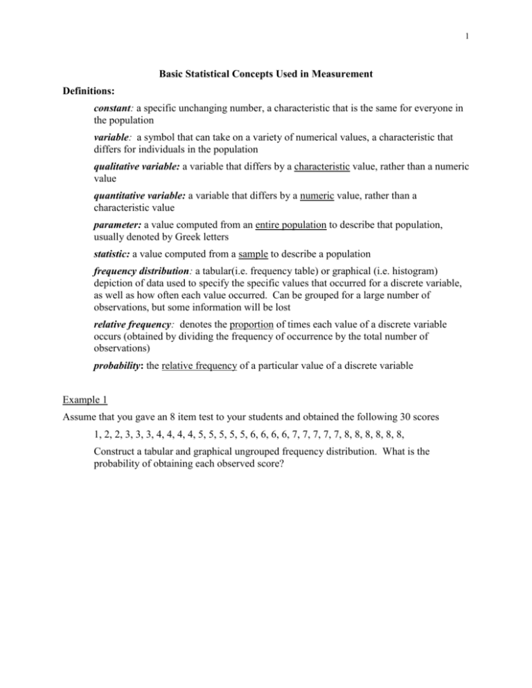
1
Basic Statistical Concepts Used in Measurement
Definitions:
constant: a specific unchanging number, a characteristic that is the same for everyone in
the population
variable: a symbol that can take on a variety of numerical values, a characteristic that
differs for individuals in the population
qualitative variable: a variable that differs by a characteristic value, rather than a numeric
value
quantitative variable: a variable that differs by a numeric value, rather than a
characteristic value
parameter: a value computed from an entire population to describe that population,
usually denoted by Greek letters
statistic: a value computed from a sample to describe a population
frequency distribution: a tabular(i.e. frequency table) or graphical (i.e. histogram)
depiction of data used to specify the specific values that occurred for a discrete variable,
as well as how often each value occurred. Can be grouped for a large number of
observations, but some information will be lost
relative frequency: denotes the proportion of times each value of a discrete variable
occurs (obtained by dividing the frequency of occurrence by the total number of
observations)
probability: the relative frequency of a particular value of a discrete variable
Example 1
Assume that you gave an 8 item test to your students and obtained the following 30 scores
1, 2, 2, 3, 3, 3, 4, 4, 4, 4, 5, 5, 5, 5, 5, 6, 6, 6, 6, 7, 7, 7, 7, 7, 8, 8, 8, 8, 8, 8,
Construct a tabular and graphical ungrouped frequency distribution. What is the
probability of obtaining each observed score?
2
summation sign:  (Greek capital letter sigma) used to symbolize the summation of
discrete variable from the lower limit (denoted at the bottom of ) to the upper limit
(denoted at the top of ).
Example: Let X represent exam scores and let Xi represent the exam score for
student i. Assume we have 5 students with the following scores: 34, 50, 41, 39,
and 45. Then:
5
X
i 1
i
 34  50  41  39  45  209 and
5
X
i 1
2
i
 34 2  50 2  412  39 2  45 2  8,883 and
2
 5

  X i   (34  50  41  39  45) 2  209 2  43,681
 i 1 
central tendency: a measure of where the center of a distribution lies - the three most
commonly used indices of central tendency are mean, median, and mode.
mean: the average of all observations, denoted by  for a population and X for a sample
N
 Xi
  i1
N
where N = the number of observations in the population

Can be thought of as the balancing point of the distribution

Is greatly affected by skewness because each and every score affects it

Is unbiased, meaning when calculating from a sample it does not
systematically over or under estimate the population mean

Is the preferred measure for test score distributions because for many of the
distributions encountered in testing it is more stable then either the median or
the mode
median: the value that half of the observations fall at or below, preferred measure of
central tendency for highly skewed distribution

Is not sensitive to the magnitude of outliers or extreme values

Is the preferred measure of central tendency with skewed distributions
mode: the most frequently occurring observation

Not a very reliable or stable measure with quantitative data

Is the preferred statistic for qualitative data
3
Example 2:
Calculate the mean, median and mode from the observed test scores given in the Example 1
variability: a measure of the degree to which observations vary – the three most
commonly used indices of variability are range, variance, and standard deviation
range: the difference between the largest and smallest observation occurring in the
distribution
deviation score: the difference, or distance, between an individual score and the group’s
mean, denoted by x (i.e. x = X - 
variance: the average squared deviation score, denoted by 2 for a population and s2 for a
sample
N
2 
 X
i 1
 
2
i
N
where N = number of observations
standard deviation: the square root of the variance (denoted by  for a population and
by s for a sample) which represents the average difference between observations and the
mean – this is usually easier to interpret because it is expressed in linear units, rather than
squared units.
Example 3:
Calculate the range, variance, and standard deviation of the observations given in the
Example 1
4
normal distribution: a theoretical symmetrical distribution for continuous variables that
follows a bell shaped curve with many observations near the middle and fewer scores at
the extreme. In this distribution the mean = median = mode
uniform distribution: a distribution for which every value has the same relative
frequency, in other words has an equal probability of occurring. This distribution has no
mode and the mean = median
positively skewed distribution: a distribution in which only a few of the observations are
in the upper range of scores. Typically in this distribution the mean > median > mode
negatively skewed distribution: a distribution in which only a few of the observations are
in the lower range of scores. Typically in this distribution the mean < median < mode
unimodal distribution: a distribution with only one mode. Most distributions are
unimodal, including the normal distribution and skewed distribution
bimodal distribution: a distribution with two modes. Many times distributions are called
bimodal even if there are not two true modes.
Describing the Relationship Between Two Variables
Pearson correlation coefficient: a measure of the linear relationship between two variables, X
and Y represented by xy for a population and rxy for a sample.
N
 xy 
(X  
i 1
X
)(Y   Y )
N X  Y

Correlation coefficients can only take on values between –1 and +1

A large negative correlation coefficient (i.e. close to –1) represents a strong negative
linear relationship while a large positive correlation (i.e. close to 1) represents a
strong positive linear relationship

A correlation close to zero represents little or no linear relationship

The square of the correlation coefficient represents how much of the variance of one
variable (say Y) is accounted for by its linear relationship with another variable

A strong correlations does not imply a causal relationship
5

Restriction of range of one or both of the observed variables causes the correlation to
be smaller than it would have been if the entire range of observations were used,
referred to as attenuation.

If the relationship between variables differs across groups and the groups are
combined then the correlation for the combined groups might be misleading
Example 4
Calculate the correlation coefficient for the following data. Note that the mean of Test A = 6, the
mean of Test B = 25.2, the standard deviation of Test A = 1.58 and the standard deviation of Test
B = 5.89
Test A
5
7
8
4
6
Test B
21
32
30
25
18