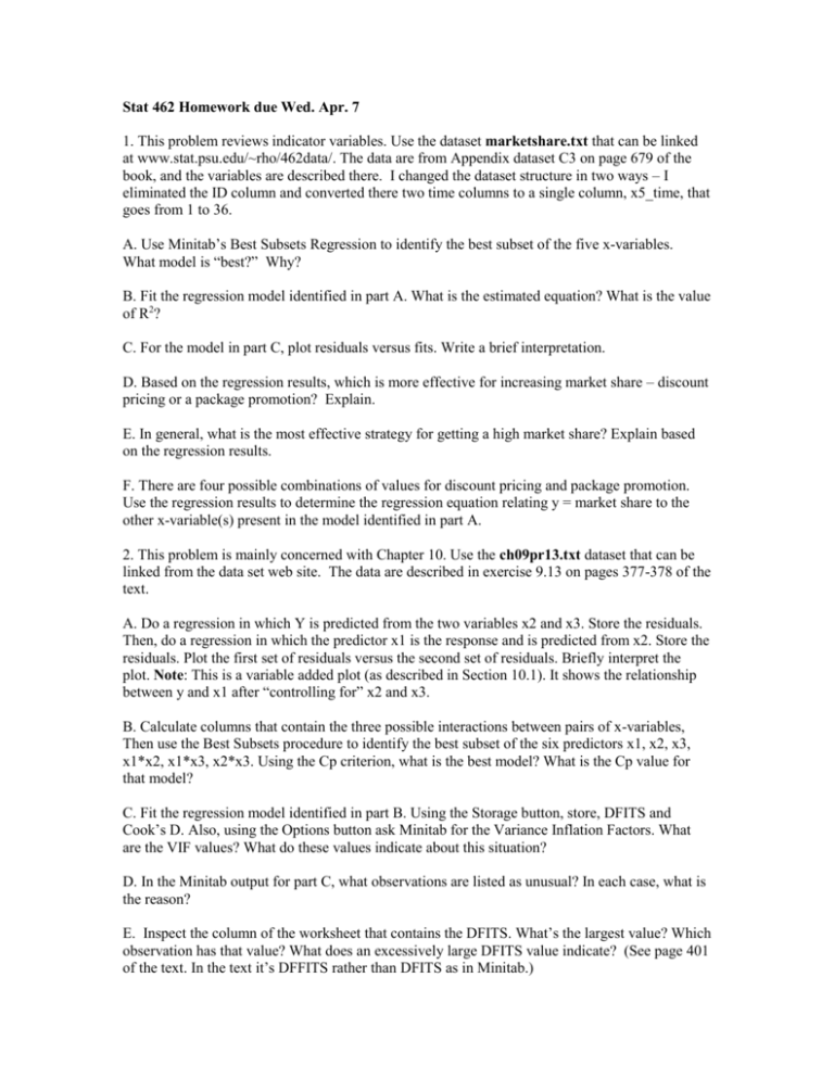
Stat 462 Homework due Wed. Apr. 7
1. This problem reviews indicator variables. Use the dataset marketshare.txt that can be linked
at www.stat.psu.edu/~rho/462data/. The data are from Appendix dataset C3 on page 679 of the
book, and the variables are described there. I changed the dataset structure in two ways – I
eliminated the ID column and converted there two time columns to a single column, x5_time, that
goes from 1 to 36.
A. Use Minitab’s Best Subsets Regression to identify the best subset of the five x-variables.
What model is “best?” Why?
B. Fit the regression model identified in part A. What is the estimated equation? What is the value
of R2?
C. For the model in part C, plot residuals versus fits. Write a brief interpretation.
D. Based on the regression results, which is more effective for increasing market share – discount
pricing or a package promotion? Explain.
E. In general, what is the most effective strategy for getting a high market share? Explain based
on the regression results.
F. There are four possible combinations of values for discount pricing and package promotion.
Use the regression results to determine the regression equation relating y = market share to the
other x-variable(s) present in the model identified in part A.
2. This problem is mainly concerned with Chapter 10. Use the ch09pr13.txt dataset that can be
linked from the data set web site. The data are described in exercise 9.13 on pages 377-378 of the
text.
A. Do a regression in which Y is predicted from the two variables x2 and x3. Store the residuals.
Then, do a regression in which the predictor x1 is the response and is predicted from x2. Store the
residuals. Plot the first set of residuals versus the second set of residuals. Briefly interpret the
plot. Note: This is a variable added plot (as described in Section 10.1). It shows the relationship
between y and x1 after “controlling for” x2 and x3.
B. Calculate columns that contain the three possible interactions between pairs of x-variables,
Then use the Best Subsets procedure to identify the best subset of the six predictors x1, x2, x3,
x1*x2, x1*x3, x2*x3. Using the Cp criterion, what is the best model? What is the Cp value for
that model?
C. Fit the regression model identified in part B. Using the Storage button, store, DFITS and
Cook’s D. Also, using the Options button ask Minitab for the Variance Inflation Factors. What
are the VIF values? What do these values indicate about this situation?
D. In the Minitab output for part C, what observations are listed as unusual? In each case, what is
the reason?
E. Inspect the column of the worksheet that contains the DFITS. What’s the largest value? Which
observation has that value? What does an excessively large DFITS value indicate? (See page 401
of the text. In the text it’s DFFITS rather than DFITS as in Minitab.)
F. Inspect the column of the worksheet that contains the Cook’s D values. What’s the largest
value? Which observation has that value? What does an excessively large Cook’s distance value
indicate? (See page 402 of the text.)
G. Turn the y-value for the most influential case into a missing value by replacing the y-value
with an asterisk in the worksheet. Fit the model identified in part B. Write the estimated equation.
Then, write the estimated equation found in part C in which all data were used. Use each
equation to predict y for the case that you deleted. For each situation (point deleted or included),
determine the predicted value for the observation that was deleted. Note: The difference between
the two values is an unstandardized version of the DFIT.
3. Use this data set:
X 1 2 3 4 5 6
Y 2 4 5 7 10 20
a. Find an unstandardized deleted residual for the 6th observation. Show how you found this.
b. Find an unstandardized deleted residual for the 3rd observation. Show how you found this.
Note: You can use Minitab for assistance.