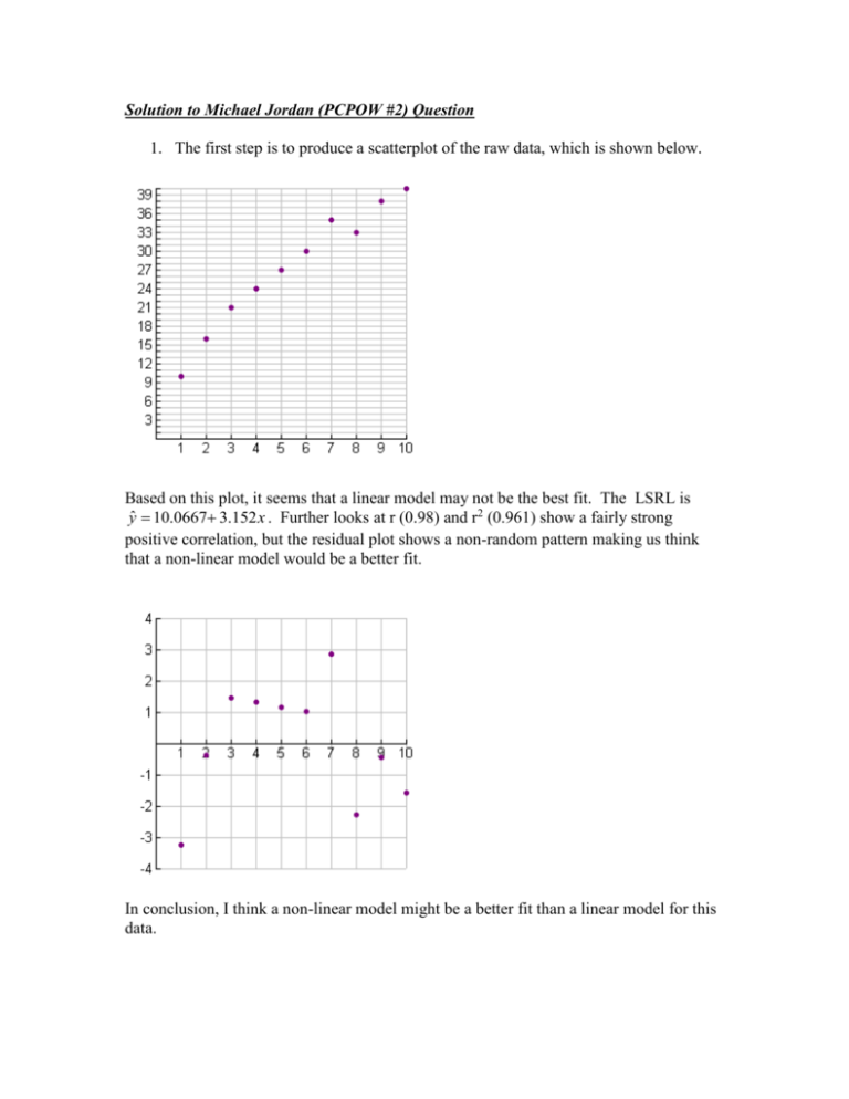
Solution to Michael Jordan (PCPOW #2) Question
1. The first step is to produce a scatterplot of the raw data, which is shown below.
Based on this plot, it seems that a linear model may not be the best fit. The LSRL is
yˆ  10.0667 3.152 x . Further looks at r (0.98) and r2 (0.961) show a fairly strong
positive correlation, but the residual plot shows a non-random pattern making us think
that a non-linear model would be a better fit.
In conclusion, I think a non-linear model might be a better fit than a linear model for this
data.
2. My equation was yˆ  10.0667 3.152 x . So y(10) = 10.0667 + 31.52 = 41.58
points. Residuals are found by taking y  y , or 40-41.58 = - 1.58
3. If we look at the ratio of his scoring outputs, we get the following:
1.6, 1.3125, 1.14, 1.125…. The final value is 1.05 and this does NOT appear to be
consistent. Thus, we dismiss the possibility of an exponential relationship and
now seek a power model.
To transform data into a power model we take the log of both x and y data sets:
Log(x)
0
0.3010299957
0.4771212547
0.6020599913
0.6989700043
0.7781512504
0.84509804
0.903089987
0.9542425094
1
Log(y)
1
1.204119983
1.322219295
1.380211242
1.431363764
1.477121255
1.544068044
1.51851394
1.579783597
1.602059991
Now we repeat the previous steps for linear regression, starting with the scatter
plot.
This certainly looks more linear than before, so we check the regression analysis.
.
The equation of the LSRL is y  0.589 x  11095
, and r = 0.9956, with r2 = 0.9913, both
significantly higher than previously.
Finally, we need to look at the residuals:
This pattern looks far more random than before, which seems to indicate these
transformed data are well-fit by a linear model.
.
Now we transform the LSRL back to power form : y  0.589 x  11095
becomes:
y  101.1095 x 0.589  10.459 x 0.589
This, then, is our working model.
4. Now, Michael’s predicted output in game 10 is y= 10.459(100.589)=40.6 points.
5. While our prediction isn’t much better, it IS better, producing a residual of –0.6
instead of –2.2 . But more importantly, our power model, once transformed, fit
the pieces of the linear regression more consistently. Namely, its scatterplot
appeared linear, its r and r2 values were quite a bit higher, and its residual plot
was notably more random than the original residuals. Thus, for all those reasons,
we can conclude that the power model is the best predictor of Michael’s future
success.
FYI – this model is essentially a square root function which grows ever more
slowly, so while Michael’s output obviously didn’t keep growing, this power
model appears to ‘flatten out’ sooner than would the linear model.
Tie breaker: Michael Jordan scored 15 points in his final appearance in an NBA
uniform, playing for the Washington Wizards at Philadelphia on April 16,
2003.