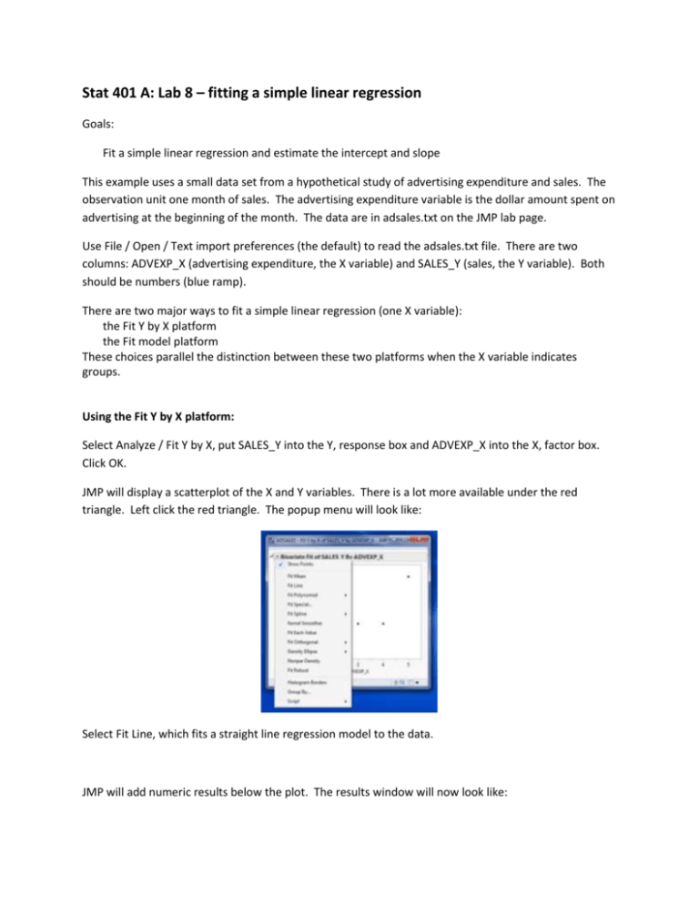
Stat 401 A: Lab 8 – fitting a simple linear regression
Goals:
Fit a simple linear regression and estimate the intercept and slope
This example uses a small data set from a hypothetical study of advertising expenditure and sales. The
observation unit one month of sales. The advertising expenditure variable is the dollar amount spent on
advertising at the beginning of the month. The data are in adsales.txt on the JMP lab page.
Use File / Open / Text import preferences (the default) to read the adsales.txt file. There are two
columns: ADVEXP_X (advertising expenditure, the X variable) and SALES_Y (sales, the Y variable). Both
should be numbers (blue ramp).
There are two major ways to fit a simple linear regression (one X variable):
the Fit Y by X platform
the Fit model platform
These choices parallel the distinction between these two platforms when the X variable indicates
groups.
Using the Fit Y by X platform:
Select Analyze / Fit Y by X, put SALES_Y into the Y, response box and ADVEXP_X into the X, factor box.
Click OK.
JMP will display a scatterplot of the X and Y variables. There is a lot more available under the red
triangle. Left click the red triangle. The popup menu will look like:
Select Fit Line, which fits a straight line regression model to the data.
JMP will add numeric results below the plot. The results window will now look like:
We have not talked about most of these numbers (but we will talk about most of them later). For now,
we need the estimated intercept and estimated slope. Those are found in two places in the results:
a. Immediately below Linear Fit, at the top of the numeric results. This is the fitted equation. Make
sure you remember which value is the intercept and which is the slope
b. In the parameter estimates box at the bottom of the results. The intercept is labelled as Intercept.
The slope is labelled by the name of the corresponding X variable (here, ADVEXP_X). That’s because
later we will have models with one intercept and multiple slopes. Labelling by the X variable uniquely
identifies each slope. The estimated values are in the estimate column.
Using the Fit model platform:
Select Analyze / Fit Model, put SALES_Y into the Y box. Use the Add button to put ADVEXP_X into the
model effects box (or drag and drop into that box). I usually change Emphasis to Minimal Report,
because I ignore most of the plots added by the default Effect Leverage. Click OK.
As with the Fit Y by X results, we will talk about most of these numbers in the next week or so.
The estimated intercept and slope are found in the Parameter Estimates box. The explanation is the
same as the explanation of that box in the Fit Y by X results.