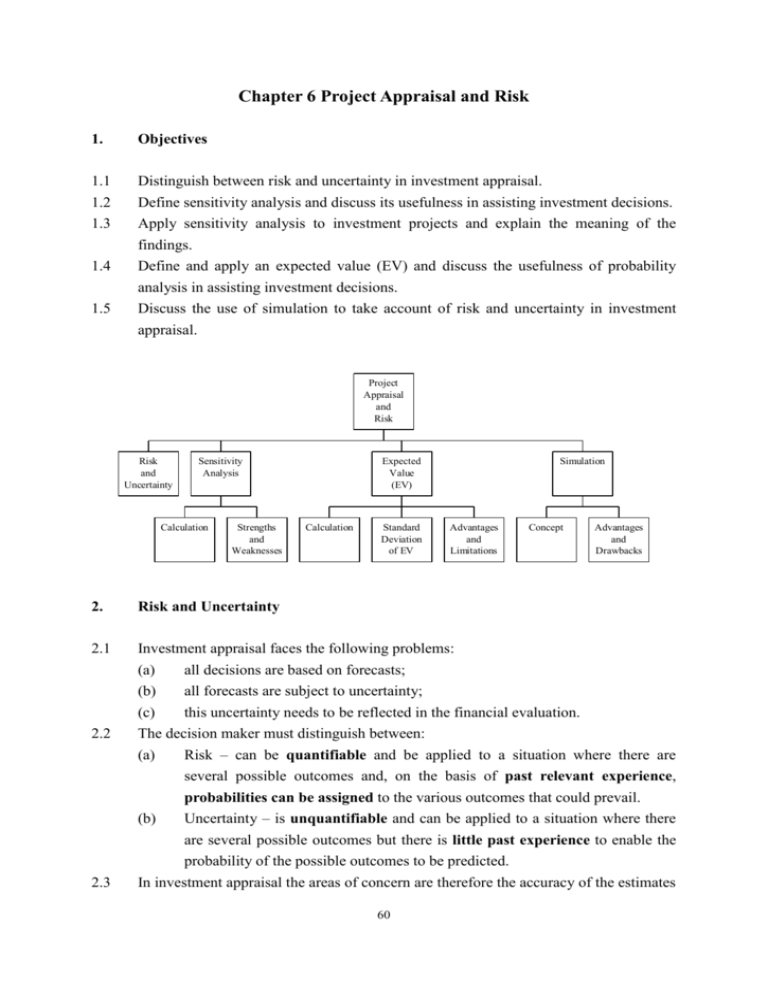
Chapter 6 Project Appraisal and Risk
1.
Objectives
1.1
1.2
1.3
Distinguish between risk and uncertainty in investment appraisal.
Define sensitivity analysis and discuss its usefulness in assisting investment decisions.
Apply sensitivity analysis to investment projects and explain the meaning of the
findings.
Define and apply an expected value (EV) and discuss the usefulness of probability
analysis in assisting investment decisions.
Discuss the use of simulation to take account of risk and uncertainty in investment
1.4
1.5
appraisal.
Project
Appraisal
and
Risk
Risk
and
Uncertainty
Sensitivity
Analysis
Calculation
Strengths
and
Weaknesses
Expected
Value
(EV)
Calculation
Standard
Deviation
of EV
Simulation
Advantages
and
Limitations
Concept
2.
Risk and Uncertainty
2.1
Investment appraisal faces the following problems:
(a)
all decisions are based on forecasts;
(b)
all forecasts are subject to uncertainty;
(c)
this uncertainty needs to be reflected in the financial evaluation.
2.2
The decision maker must distinguish between:
Risk – can be quantifiable and be applied to a situation where there are
several possible outcomes and, on the basis of past relevant experience,
probabilities can be assigned to the various outcomes that could prevail.
(b)
Uncertainty – is unquantifiable and can be applied to a situation where there
are several possible outcomes but there is little past experience to enable the
probability of the possible outcomes to be predicted.
In investment appraisal the areas of concern are therefore the accuracy of the estimates
(a)
2.3
Advantages
and
Drawbacks
60
concerning:
(a)
(b)
(c)
Project life
Predicted cash flows and associated probabilities
Discount rate used
3.
Sensitivity Analysis
3.1
Sensitivity analysis typically involves posing “what if?” questions. For example, what
if demand fell by 10% compared to our original forecasts? Would the project still be
viable?
3.2
In project appraisal, sensitivity analysis assesses how responsive the project’s NPV
3.3
is to changes in the variables used to calculate that NPV.
The NPV could depend on a number of uncertain independent variables.
(a)
Selling price
3.4
3.5
(b)
Sales volume
(c)
Cost of capital
(d)
Initial cost
(e)
Operating costs
(f)
Benefits
Sensitivity analysis therefore provides an indication of why a project might fail.
Management should review critical variables to assess whether or not there is a strong
possibility of events occurring which will lead to a negative NPV. Management should
also pay particular attention to controlling those variables to which the NPV is
particularly sensitive, once the decision has been taken to accept the investment.
A simple approach to deciding which variables the NPV is particularly sensitive to is
to calculate the sensitivity of each variable:
Sensitivity
3.6
=
NPV
PV of project variable
%
The lower the percentage, the more sensitive is NPV to that project variable as the
variable would need to change by a smaller amount to make the project non-viable.
61
3.7
EXAMPLE 1
ABC Co is considering a project with the following cash flows.
Year
Initial
Variable costs
Cash inflows
Net cash flows
investment
($000)
($000)
($000)
1
(2,000)
6,500
4,500
2
(2,000)
6,500
4,500
($000)
0
7,000
Cash flows arise from selling 650,000 units at $10 per unit. ABC Co has a cost of
capital of 8%.
Required:
Measure the sensitivity of the project to changes in variables.
Solution:
The PVs of the cash flow are as follows.
Year
Discount
PV of initial
PV of
PV of cash
PV of net
factor 8%
investment
variable costs
inflows
cash flow
$000
$000
$000
$000
0
1.000
(7,000)
(7,000)
1
0.926
(1,852)
6,019
4,167
2
0.857
(1,714)
5,571
3,857
(3,566)
11,590
1,024
(7,000)
NPV = 1,024
The project has a positive NPV and would appear to be worthwhile. The sensitivity
of each project variable is as follows.
(a)
Initial investment
Sensitivity = 1,024 / 7,000 x 100% = 14.6%
(b)
Sales volume
Sensitivity = 1,024 / (11,590 – 3,566) x 100% = 12.8%
62
(c)
Selling price
Sensitivity = 1,024 / 11,590 x 100% = 8.8%
(d)
Variable costs
Sensitivity = 1,024 / 3,566 x 100% = 28.7%
(e)
Cost of capital. We need to calculate the IRR of the project.
Year
Net cash
Discount
flow
factor 15%
PV
Discount
PV
factor 20%
$000
$000
$000
0
(7,000)
1
(7,000)
1
(7,000)
1
4,500
0.870
3,915
0.833
3,749
2
4,500
0.756
3,402
0.694
3,123
317
(128)
 317

 (0.2  0.15) = 18.56%
IRR = 0.15 + 
 317  128

The cost of capital can therefore increase by 133% before the NPV becomes
negative.
The elements to which the NPV appears to be most sensitive are the selling price
followed by the sales volume. Management should thus pay particular attention to
these factors so that they can be carefully monitored.
3.8
Strengths and weaknesses of sensitivity analysis
Strengths
(a)
(b)
(c)
No
complicated
Weaknesses
theory
to (a)
understand.
Information will be presented to
management in a form which
facilitates subjective judgement to
decide the likelihood of the
various
possible
outcomes
considered.
Identifies areas which are crucial
63
It
assumes
that
changes
to
variables
can
be
made
independently, e.g. material prices
will change independently of
other variables. This is unlikely. If
material prices went up the firm
would probably increase selling
price at the same time and there
would be little effect on NPV. A
(d)
to the success of the project. If the
technique called simulation (see
project is chosen, those areas can
be carefully monitored.
Indicates just how critical are (b)
some of the forecasts which are
considered to be uncertain.
later) allows us to change more
than one variable at a time.
It only identifies how far a
variable needs to change. It does
not look at the probability of such
a change. In the above analysis,
sales volume appears to be the
most crucial variable, but if the
firm were facing volatile raw
material markets a 65% change in
raw material prices would be far
more likely than a 29% change in
sales volume.
(c)
It is not an optimising technique.
It provides information on the
basis of which decisions can be
made. It does not point directly to
the correct decision.
4.
Expected Value (EV)
4.1
When there are a number of possible outcomes for a decision and probabilities can be
assigned to each, then an EV may be calculated.
4.2
CONCEPT
The EV is the weighted average of all possible outcomes, with the weightings
based on the probability estimates.
The formula for calculating an EV is:
EV =
 px
Where: p = the probability of an outcome
x = the value of an outcome
64
4.3
EXAMPLE 2
A firm has to choose between three mutually exclusive, the outcomes of which
depend on the state of the economy. The following estimates have been made:
State of the
economy
Probability
Project A
Project B
Project C
Recession
Stable
Growing
0.5
NPV ($000)
100
0
180
0.4
NPV ($000)
200
500
190
0.1
NPV ($000)
1,400
600
200
Determine which project should be selected on the basis of expected market values.
Solution:
Project A
State of the economy
Recession
Stable
Growing
Probability
Project NPV
$000
EV
$000
0.5
0.4
0.1
100
200
1,400
50
80
140
270
Project B
State of the economy
Probability
Recession
Stable
0.5
0.4
Project NPV
$000
0
500
Growing
0.1
600
EV
$000
0
200
60
260
Project C
State of the economy
Recession
Stable
Probability
0.5
0.4
65
Project NPV
$000
180
190
EV
$000
90
76
Growing
0.1
200
20
186
On the basis of expected values, Project A should be selected.
However, it should be noted that Project A is also the most risky option as it has the
widest range of potential outcomes.
4.4
EXAMPLE 3
ABC Co is considering an investment of $460,000 in a non-current asset expected
to generate substantial cash inflows over the next five years. Unfortunately the
annual cash flows from this investment are uncertain, but the following probability
distribution has been established:
Annual cash flow ($)
50,000
100,000
150,000
Probability
0.3
0.5
0.2
At the end of its five-year life, the asset is expected to sell for $40,000. The cost of
capital is 5%.
Should the investment be undertaken?
Solution:
Expected annual cash flows are:
Annual cash flow
50,000
100,000
150,000
Probability
0.3
0.5
0.2
EV
15,000
50,000
30,000
95,000
NPV calculation:
Time
0
1
2
Cash flow
(460,000)
95,000
40,000
DF 5%
1.000
4.329
0.784
NPV =
66
PV
(460,000)
411,255
31,360
(17,385)
As the ENPV is negative, the project should not be undertaken.
An alternative approach would be to calculate three separate NPVs and then
combine them, giving the following figures:
Annual cash flow
50,000
100,000
150,000
Probability
0.3
0.5
0.2
PV
(212,190)
4,260
220,710
ENPV = 0.3 x (212,190) + 0.5 x 4,260 + 0.2 x 220,710 = (17,385)
Even though the ENPV is negative these figures show that there is a 70% chance of
the project giving a positive NPV. Some investors may consider the project
acceptable on this basis.
4.5
Test your understanding 1
A company is considering whether to invest in equipment for providing a new
service to its clients. The equipment will cost $100,000 and will have a disposal
value of $20,000 after four years. Estimates of sales and incremental fixed cost
cash expenditures are as follows.
Annual cash flow ($)
600,000
700,000
800,000
Probability
0.4
0.4
0.2
The company expects to achieve a contribution/sales ratio of 40% on all the
services it provides. Incremental fixed costs will be $215,000 per annum. The
project has a four-year life.
The company’s cost of capital is 9%.
Calculate the three possible NPVs an the expected NPV. Comment on your results.
67
Solution:
68
4.6
EXAMPLE 4
A company is considering a project involving the outlay of $300,000 which it
estimates will generate cash flows over its two year life at the probabilities shown
in the following table.
Year 1
Annual cash flow ($)
100,000
200,000
300,000
Probability
0.25
0.50
0.25
Year 2
If cash flows in Year 1
There is probability of:
is:
That the cash flow in
Year 2 will be:
100,000
200,000
300,000
0.25
Nil
0.50
100,000
0.25
200,000
0.25
100,000
0.50
200,000
0.25
300,000
0.25
200,000
0.50
300,000
0.25
350,000
The company’s investment criterion for this type of project is 10% DCF.
You are required to calculate the expected value of the project’s NPV and the
probability that the NPV will be negative.
Solution:
Calculate expected value of the NPV.
First we need to draw up a probability distribution of the expected cash flows. We
begin by calculating the PV of the cash flows.
Year
Cash flow
$000
DF 10%
69
PV
$000
1
100
0.909
90.9
1
1
2
2
2
2
200
300
100
200
300
350
0.909
0.909
0.826
0.826
0.826
0.826
181.8
272.7
82.6
165.2
247.8
289.1
Year 1
Prob.
Year 2
PV of
PV of
cash
cash
flow
flow
$000
$000
Prob.
Joint
Total PV
EV of
Prob.
of cash
PV of
inflows
cash
inflows
$000
$000
(a)
(b)
(c)
(d)
(b) x (d)
(a) + (c)
90.9
0.25
0.0
0.25
0.0625
90.9
5.681
90.9
0.25
82.6
0.50
0.125
173.5
21.688
90.0
0.25
165.2
0.25
0.0625
256.1
16.006
181.8
0.50
82.6
0.25
0.125
264.4
33.05
181.8
0.50
165.2
0.50
0.250
347
86.75
181.8
0.50
247.8
0.25
0.125
429.6
53.70
272.7
0.25
165.2
0.25
0.0625
437.9
27.369
272.7
0.25
247.8
0.50
0.125
520.5
65.063
272.7
0.25
289.1
0.25
0.0625
561.8
35.113
344.420
EV of PV of cash inflows
Less: Project cost
$
344,420
300,000
EV of NPV
44,420
Measure risk.
Since the EV of the NPV is positive, the project should go ahead unless the risk is
unacceptably high. The probability that the project will have a negative NPV is the
probability that the total PV of cash inflows is less than $300,000. From the column
headed ‘Total PV of cash inflows’, we can establish that this probability is 0.0625 +
0.125 + 0.0625 + 0.125 = 0.375 or 37.5%. This might be considered an
unacceptably high risk.
70
(A)
The standard deviation of the NPV
4.7
The disadvantage of using the EV of NPV approach to assess the risk of the project is
that the construction of the probability distribution can become very complicated.
If we were considering a project over 4 years, each year have five different forecasted
cash flows, there would be 625 (54) NPVs to calculate. To avoid all of these
calculations, an indication of the risk may be obtained by calculating the standard
deviation of the NPV.
4.8
EXAMPLE 5
Frame Co is considering which of two mutually exclusive projects, A or B, to
undertake. There is some uncertainty about the running costs with each project, and
a probability distribution of the NPV for each project has been estimated, as
follows.
Project A
NPV
$000
– 20
+ 10
Probability
Probability
0.15
0.20
Project B
NPV
$000
+5
+ 15
+ 20
+ 40
0.35
0.30
+ 20
+ 25
0.4
0.1
0.2
0.3
You are required to decide which project should the company choose, if either.
Solution:
We can begin by calculating the EV of the NPV for each project.
Project A
NPV
$000
– 20
10
20
40
Prob.
0.15
0.20
0.35
0.30
Project B
EV
$000
(3.0)
2.0
7.0
12.0
NPV
$000
5
15
20
25
18.0
Prob.
0.2
0.3
0.4
0.1
EV
$000
1.0
4.5
8.0
2.5
16.0
71
Project A has a higher EV of NPV, but what about the risk of variation in the NPV
above or below the EV? This can be measured by the standard deviation of the
NPV.
The standard deviation of a project’s NPVs, can be calculated as:
 p ( x  x)
s
x
– 20
2
, where x is the EV of the NPV.
Project A, x = 18
p
x- x
p(x - x )2
0.15
– 38
216.6
10
0.20
20
0.35
40
0.30
–8
+2
+ 22
5
Project B, x = 16
p
x- x
p(x - x )2
0.2
– 11
24.2
12.8
15
0.3
1.4
20
0.4
145.2
25
0.1
x
–1
+4
+9
376.0
0.3
6.4
8.1
39.0
Project A
Standard deviation
Project B
Standard deviation
s = 376 = 19.391
= $19,391
s = 39.0 = 6.245
= $6,245
Although Project A has a higher EV of NPV, it also has a higher standard deviation
of NPV, and so has greater risk associated with it.
Which project should be selected? Clearly it depends on the attitude of the
company’s management to risk.
4.9
(a)
If management are prepared to take the risk of a low NPV in the hope of a
high NPV they will opt for project A.
(b)
If management are risk-averse, they will opt for the less risky project B.
Advantages and limitation of expected values
Advantages
(a)
Limitations
The technique recognises that (a)
there
are
several
possible
outcomes and is, therefore, more
sophisticated than single value
forecasts.
72
By asking for a series of forecasts
the whole forecasting procedure is
complicated.
Inaccurate
forecasting is already a major
weakness in project evaluation.
(b)
Enables the probability of the
The probabilities used are also
(c)
different
outcomes
to
be
quantified.
(b)
Leads directly to a simple
optimising decision rule.
Calculations are relatively simple.
usually very subjective.
The EV is merely a weighted
average of the probability
distribution,
indicating
the
average payoff if the project is
repeated many times.
The EV gives no indication of the
dispersion of possible outcomes
about the EV. The more widely
spread out the possible results are,
(d)
(c)
the more risky the investment is
usually seen to be. The EV
ignores this aspect of the
(d)
probability distribution.
In ignoring risk, the EV technique
also ignores the investor’s attitude
to risk. Some investors are more
likely to take risks than others.
5.
Simulation (模擬)
5.1
Sensitivity analysis considered the effect of changing one variable at a time.
Simulation improves on this by looking at the impact of many variables changing
at the same time.
Using mathematical, it produces a distribution of the possible outcomes from the
project. The probability of different outcomes can then be calculated.
5.2
5.3
EXAMPLE 6
The following probability estimates have been prepared for a proposed project.
Year
Probability
Cost of equipment
0
1.00
(40,000)
Revenue each year
1–5
0.15
40,000
0.40
50,000
0.30
55,000
0.15
60,000
73
1–5
Running costs each year
0.10
25,000
0.25
30,000
0.35
35,000
0.30
40,000
The cost of capital is 12%. Assess how a simulation model might be used to assess
the project’s NPV.
Solution:
A simulation model could be constructed by assigning a range of random number
digits to each possible value for each of the uncertain variables. The random
numbers must exactly match their respective probabilities. This is achieved by
working upwards cumulatively from the lowest to the highest cash flow values and
assigning numbers that will correspond to probability groupings as follows.
Revenue
$
Prob.
Running costs
Random
$
Prob.
No.
Random
No.
40,000
0.15
00 – 14
*
25,000
0.10
00 – 09
50,000
0.40
15 – 54
**
30,000
0.25
10 – 34
55,000
0.30
55 – 84
***
35,000
0.35
35 – 69
60,000
0.15
85 – 99
40,000
0.30
70 – 99
* Probability is 0.15 (15%). Random numbers are 15% of range 00 – 99.
** Probability is 0.40 (40%). Random numbers are 40% of range 00 – 99 but
starting at 15.
*** Probability is 0.30 (30%). Random numbers are 30% of range 00 – 99 but
starting at 55.
For revenue, the selection of a random number in the range 00 and 14 has a
probability of 0.15. This probability represents revenue of $40,000. Numbers have
been assigned to cash flows so that when numbers are selected at random, the cash
flows have exactly the same probability of being selected as is indicated in their
respective probability distribution above.
Random numbers would be generated, for example by a computer program, and
these would be used to assign values to each of the uncertain variables.
74
For example, if random numbers 378420015689 were generated, the values
assigned to the variables would be as follows.
Revenue
Calculation
Random No.
Running costs
Value
Random No.
$
Value
$
1
37
50,000
84
40,000
2
20
50,000
01
25,000
3
56
55,000
89
40,000
A computer would calculate the NPV many times over using the values established
in this way with more random numbers, and the results would be analysed to
provide the following.
(a)
(b)
An expected value for the project.
A statistical distribution pattern for the possible variation in the NPV above
or below this average.
The decision whether to go ahead with the project would then be made on the basis
of expected return and risk.
5.4
Advantages and drawbacks of simulation
Advantages
(a)
(b)
(c)
Drawbacks
It includes all possible outcomes in (a)
the decision-making process.
It is a relatively easily understood
technique.
It has a wide variety of
Models can become extremely
complex and the time and costs
involved in their construction can
be more than is gained from the
improved decisions.
applications (inventory control, (b)
component replacement, etc.)
Probability distributions may be
difficult to formulate.
75
Examination Style Questions
Question 1 – NPV and Sensitivity Analysis
Betula Co has recently acquired a patent, at a cost of $1·3 million, which would allow it to
manufacture and sell a product for measuring an individual’s bio-rhythms. The marketing
department of Betula Co estimates that 300,000 units of this product can be sold during each
of the next four years. The selling price of the product is $24 and variable costs are estimated
to be $18 per product. Fixed costs (excluding depreciation) are estimated to be $2·2 million
per year. This figure consists of $1·4 million additional fixed costs and $0·8 million existing
fixed costs that are to be apportioned to the new product.
To manufacture the new product, equipment costing $1·5 million will be acquired
immediately. The estimated residual value of this equipment in four years’ time is $0·5
million. The company calculates depreciation on a straight-line basis.
The cost of capital of Betula Co is 9%.
Betula is currently considering whether to go ahead with the project.
Required:
(a)
(b)
(c)
Calculate the net present value of the decision to go ahead with the project.
(5 marks)
Undertake sensitivity analysis to show the change needed to each of the following
before a zero NPV is achieved:
(i) discount rate;
(ii) initial outlay on equipment;
(iii) net annual operating cash flows;
(iv) residual value of the equipment.
(11 marks)
Evaluate briefly the information produced in your answer to (a) and (b) above and state,
with reasons, whether or not the project should go ahead.
(4 marks)
(Total 20 marks)
76
Question 2 – Expected value and Working Capital Management
ZSE Co is concerned about exceeding its overdraft limit of $2 million in the next two periods.
It has been experiencing considerable volatility in cash flows in recent periods because of
trading difficulties experienced by its customers, who have often settled their accounts after
the agreed credit period of 60 days. ZSE has also experienced an increase in bad debts due to
a small number of customers going into liquidation.
The company has prepared the following forecasts of net cash flows for the next two periods,
together with their associated probabilities, in an attempt to anticipate liquidity and financing
problems. These probabilities have been produced by a computer model which simulates a
number of possible future economic scenarios. The computer model has been built with the
aid of a firm of financial consultants.
Period 1 cash flow
$000
8,000
4,000
(2,000)
Probability
10%
60%
30%
Period 2 cash flow
$000
7,000
3,000
(9,000)
Probability
30%
50%
20%
ZSE Co expects to be overdrawn at the start of period 1 by $500,000.
Required:
(a)
Calculate the following values:
(i) the expected value of the period 1 closing balance;
(ii) the expected value of the period 2 closing balance;
(iii) the probability of a negative cash balance at the end of period 2;
(iv) the probability of exceeding the overdraft limit at the end of period 2.
Discuss whether the above analysis can assist the company in managing its cash flows.
(13 marks)
(b)
Identify and discuss the factors to be considered in formulating a trade receivables
management policy for ZSE Co.
(8 marks)
Discuss whether profitability or liquidity is the primary objective of working capital
management.
(4 marks)
(Total 25 marks)
(ACCA F9 Financial Management June 2010 Q1)
(c)
77