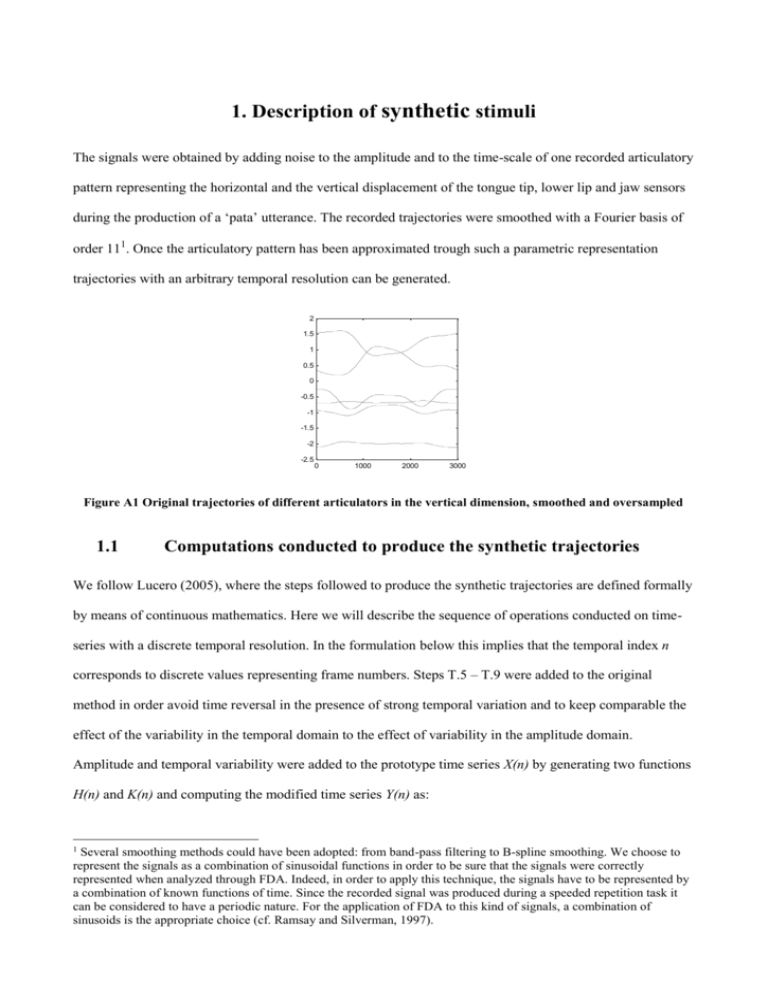
1. Description of synthetic stimuli
The signals were obtained by adding noise to the amplitude and to the time-scale of one recorded articulatory
pattern representing the horizontal and the vertical displacement of the tongue tip, lower lip and jaw sensors
during the production of a ‘pata’ utterance. The recorded trajectories were smoothed with a Fourier basis of
order 111. Once the articulatory pattern has been approximated trough such a parametric representation
trajectories with an arbitrary temporal resolution can be generated.
2
1.5
1
0.5
0
-0.5
-1
-1.5
-2
-2.5
0
1000
2000
3000
Figure A1 Original trajectories of different articulators in the vertical dimension, smoothed and oversampled
1.1
Computations conducted to produce the synthetic trajectories
We follow Lucero (2005), where the steps followed to produce the synthetic trajectories are defined formally
by means of continuous mathematics. Here we will describe the sequence of operations conducted on timeseries with a discrete temporal resolution. In the formulation below this implies that the temporal index n
corresponds to discrete values representing frame numbers. Steps T.5 – T.9 were added to the original
method in order avoid time reversal in the presence of strong temporal variation and to keep comparable the
effect of the variability in the temporal domain to the effect of variability in the amplitude domain.
Amplitude and temporal variability were added to the prototype time series X(n) by generating two functions
H(n) and K(n) and computing the modified time series Y(n) as:
1
Several smoothing methods could have been adopted: from band-pass filtering to B-spline smoothing. We choose to
represent the signals as a combination of sinusoidal functions in order to be sure that the signals were correctly
represented when analyzed through FDA. Indeed, in order to apply this technique, the signals have to be represented by
a combination of known functions of time. Since the recorded signal was produced during a speeded repetition task it
can be considered to have a periodic nature. For the application of FDA to this kind of signals, a combination of
sinusoids is the appropriate choice (cf. Ramsay and Silverman, 1997).
Y (n)  X ( H (n))  K (n)
(1)
As we can see from eq. (1), H(n) is a time-warping function which transforms the positions in time of the
values of X. Since the temporal resolution of the recorded time series is discrete, the output of H(n) has to be
converted to discrete values representing frame numbers. In order to limit the round off error due to the
quantization and avoid a discontinuous time-warping, the processing which follows is conducted on signals
having a temporal resolution which is 7 times the original 300 Hz sampling rate (this scaling factor was set
through visual inspection of the resulting time-series and therefore is specific to the motion patterns
processed). The prototype time-series is generated at that resolution from the parametrical representation, it
is modified, and then it is downsampled to a consistent number of samples.
Each of the six prototype curves is also normalized in amplitude (each value is subtracted from the mean
specific to that curve and the result is divided by the standard deviation). In that way, the variability added to
each articulatory dimension is scaled proportionally to the amount of movement observed in that dimension.
Once the noisy trajectories computed, the original amplitude scale is restored by adding the original mean
and multiplying by the original standard deviation. As a consequence of this manipulation, the amplitude
values in the following steps represent units of standard deviation of the original trajectories.
1.2.
Amplitude variability
The amount of amplitude variability introduced is controlled by the amplitude variability coefficient β.
A.1) A set of random numbers from a uniform distribution with range [0, 1] and length equal to the length of
the time series is generated. (cf. top panel of Figure A2).
4
2
0
-2
-4
0
500
1000
1500
2000
2500
3000
0.4
0.2
0
-0.2
-0.4
0
500
1000
1500
2000
2500
3000
Figure A2: In the top panel it is shown a random time series. In the bottom panel, the same time series is
smoothed (dashed line) and scaled (continuous line)
A.2) The random time series is then smoothed to give the amplitude noise function K(0)(n) (dashed line in the
bottom panel of Figure A2). The smoothing process forces the time series to be 0 at the beginning and at the
end. These constraints are only needed when adding variability on the time axis (and therefore are discussed
later); they are used here to keep comparable the variability in the two domains. This and the former step are
repeated for each different dimension of the prototype time-series, thus obtaining a multivariate noise
function: K(0)(n, q); where n varies across the time-frames and q varies across the different dimensions.
A.3) In order to control the amount of amplitude noise, we first computed Y(K)(n,q)=K(0)(n, q)+X(n,q) then
we subtracted Y(K)(n) from the prototype time-series. The final amplitude noise function K(n, q) (the
continuous line in the bottom panel of Figure A2) is obtained multiplying K(0)(n, q) by the coefficient β and
dividing from the average error computed over the difference between K(0)(n, q) and X(n,q).
K ( n) 
K ( 0) (n).
1 N Q

NQ n1 q1
X (n, q)  Y
(K )
(n, q)

(2)
2
Here N indicates the number of points of the two time series and Q indicates the number of dimensions.
K(n,q) is then added to the prototype once its time scale has been modified (cf. step T.8).
1.3. Temporal variability
The amount of temporal variability introduced is controlled by the coefficient γ.
T.1) As for the amplitude variation, a random time-series J(0)(n) is created by sampling the appropriate
number of random values from a uniform distribution within the interval [0,…,1].
T.2) J is obtained by smoothing J(0)(n) through Bspline smoothing with the following boundary constraints:
J(1) = J(N) = D( J(1) ) = D( J(N) ) = 0, where D(J(N)) is the time derivative of J at frame n and N indicates
the total number of frames of the time series. These constraints assure that the edge portions of the prototype
trajectory are present even in the modified trajectories.
T.3) From J we obtain the function H(0)(n).
H ( 0 ) ( n)  n   ( n)
(3)
where Φ(n) is given by:
n
 (n)   J (i )
(4)
i 1
At frame n, H(0)(n) is equal to n plus the sum of all the values of J(i), with i varying in the interval [1,…,n]
(cf. Figure A3). A new trajectory can then be derived from the prototype trajectory by:
Y ( 0) (n)  X ( H ( 0) (n))
(5)
In other words, Y(0) can be constructed by choosing the values from the original trajectory (X), in the order
specified by H(0)(n). A frame which is at position H(0)(n) in the prototype is shifted at position n in the new
trajectory.
3000
2500
2000
1500
1000
500
0
0
500
1000
1500
2000
2500
3000
Figure A3 Mapping ( H0(n) ) from frames in the prototype to frames in the time-warped trajectory.
T.4) For each point of H(0)(n), we compute the deviation from the straight line connecting the first and the
last values of H(0)(n). We obtain the function S(0)(n) which, at each time-frame, represents the temporal shift
between the new trajectory and prototype (cf. Figure A4).
0
-2
-4
-6
-8
0
500
1000
1500
2000
2500
3000
Figure A4 S0(n) represents the temporal shift among the corresponding frames in the prototype and in the timewarped time-series.
T.5) In order to control the amount of temporal variability, we proceeded as in step A.3. We computed the
error between the prototype trajectory and its warped version (Y(H)). We then multiplied S(0)(n) by gamma and
divided by the average error measure:
S ( n) 
S ( 0) (n).
1 N Q

NQ n1 q1
X (n, q)  Y
(H )
(n, q)
(6)

2
Where the index n ranges from 1 to the length of the time-series and represents the different frames, while
the index q represents the different dimensions.
T.6) A new mapping function H(n) is obtained by adding to S(n) a line of slope one.
3000
2500
2000
1500
1000
500
0
0
500
1000
1500
2000
2500
3000
Figure A5 Final mapping among frames of the prototype and of the deformed trajectories.
T.7) The mapping function H(n) has to be a monotonically increasing function because, if this function has a
locally negative slope, portions of the prototype trajectory are reversed in the trajectory with the modified
time scale. If negative slope values are found in H(n), steps T(1)-T(6) are repeated.
T.8) Once that K(n) and H(n) are available, the modified time series Y is obtained by applying eq. (1).
2
1
0
-1
-2
0
500
1000
1500
2000
2500
3000
Figure A6 The dashed line represents the prototype trajectory for vertical displacement of the jaw. The
continuous line represents the transformed trajectories obtained through the steps A.1- A.3 and T.1-T.8.
1.5. Groups of stimuli
The parameters manipulated to obtain the synthetic trajectories are the variability coefficients, for which we
choose six values ranging in equal steps between 0.035 and 0.5. We built 12 combinations of parameter
values by varying one variability coefficient and keeping the other constant at its lowest value (cf. Figure 4
in the main paper). From each parameter combination we built a set of 60 trajectories.
2.
Cleaning algorithm
Denote each group of connected recurrence points in the CRP by where
and
is the number
of the groups. These groups of recurrence points are identified through connected components labeling (see
Rosenfeld and Pfaltz; 1966). A CRP corresponds to a binary matrix of 0s and 1s; for each group of
connected points , denote by
the smallest sub matrix containing all the recurrence points belonging to the
group.
Each group of connected recurrence points potentially populates a portion of the LOS which is extracted by
applying the following steps based on the recursive algorithm of Marwan et al. (2002)to extract the LOS
from a CRP. Here we apply the algorithm separately to each submatrix
.In the following we denote by
LOS a portion of the LOS extracted from a group of connected recurrence points.
Denote all recurrence points in a group of M connected recurrence points by
and the recurrence points belonging to the LOS by
points belonging to the LOS).
(with
(with
)
and N equal to the number of
Before applying the recursive part of the algorithm, the starting point of the LOS is determined by choosing
the recurrence point which is found closest to Ql(1,1)(this is the bottom left corner of the submatrix
including the connected recurrence points).
The recursive part of the algorithm populates a (
the previous recurrence point
) submatrix in
whose (1,1)-location corresponds to
. Let W denote this sub matrix. The initial size of W is (
) and it is
increased in steps of one in both directions until W includes at least another recurrence point or until one of
the margins of
is reached. When W includes more recurrence points, we compute the center of mass of the
coordinates of the recurrence points contained by W. We set the second point of the LOS (denoted by
) at the coordinates resulting from the computation of the center of mass:
Where
are
recurrence points such that
<
<
, and
<
<
. The correction based
on the center of mass prevents the algorithm from placing the LOS on the upper edge of a group of connected
dots. However, to avoid the introduction of gaps, we deviate from the original algorithm proposed by
Marwan et al. by setting
and
point has been found, a new (
recurrence point
right or the top side of
. Once the new recurrence
) submatrix is populated whose (1,1)-location corresponds to the
and the procedure is repeated. The algorithm terminates when the LOS reaches the
. Note that the repositioning of the submatrix W at each iteration imposes a positive
monotonic constraint on the tracking, meaning that the LOS moves in the upward right direction. We can
constrain the LOS to move in the downward right direction if, at each step of the iteration, W is positioned
with its (1+w,1)-location at
(the previous recurrence point belonging to the LOS). Extracting the LOS
with a negative monotonic constraint is useful to eliminate from the plot the groups of connected recurrence
points oriented toward the bottom right direction. This is achieved by comparing the lengths of the LOSs
obtained with increasing and decreasing constraints. Groups of recurrence points producing longer LOSs
when processed with a negative monotonic constraint are discarded from the plot because it is reasonable to
assume that those groups of connected dots are originally oriented toward the bottom right direction.