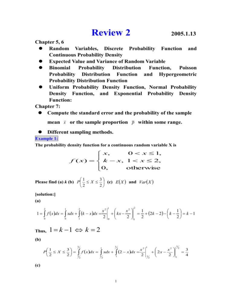
Review 2
2005.1.13
Chapter 5, 6
 Random Variables, Discrete Probability Function and
Continuous Probability Density
 Expected Value and Variance of Random Variable
 Binomial Probability Distribution Function, Poisson
Probability Distribution Function and Hypergeometric
Probability Distribution Function
 Uniform Probability Density Function, Normal Probability
Density Function, and Exponential Probability Density
Function:
Chapter 7:
 Compute the standard error and the probability of the sample
mean x or the sample proportion p within some range.
 Different sampling methods.
Example 1:
The probability density function for a continuous random variable X is
0  x  1,
 x,

f ( x )   k  x, 1  x  2,
0,
otherwise

3
1
Please find (a) k (b) P  X   (c) E X  and Var X 
2
2
[solution:]
(a)
2
1 
0
Thus,
1
2
x2
f x dx   xdx   k  x dx 
2
0
1
1
0
2

x2 
1
1

  kx     2k  2   k    k  1
2 1 2
2


1  k 1  k  2
(b)
3
1
P  X   
2
2
3
2

1
2
1
3
x2
f x dx   xdx   2  x dx 
2
1
1
2
2
(c)
1
3
1
1
2
2

x2 
3

  2 x 

2 1
4

2
1
2
x3
  E  X    xf x dx   x dx   x2  x dx 
3
0
0
1
1
2
0
2

x3 
  x 2    1 .
3 1

Since
 
E X2
1
2
 2x3 x 4 
x4
7
  x 2 f x dx   x 3 dx   x 2 2  x dx 
 
   ,
4 0  3
4 1 6
0
0
1
2
1
2
 
Var  X   E X 2   2 
7
1
 12  .
6
6
Example 2:
Twenty percent of the applications received for a particular position are rejected.
What is the probability that among the next fourteen applications,
(a) none will be rejected?
(b) all will be rejected?
(c) less than 2 will be rejected?
(d) more than one will be rejected?
(e) Determine the expected number of rejected applications and its variance.
[solution:]
Let X represent the number of rejections among the next fourteen applications.
Then, the distribution function of X is
 n
14 
n i
f i     p i 1  p    (0.2) i (0.8)14i , i  0,1,,14;
i
i
14 
 0.20 0.814  0.814  0.044




P
X

0

f
0

(a)
0
14 
 0.214 0.80  0.214  0




P
X

14

f
14

(b)
14 
(c)
P X  2   P X  0   P  X  1  f 0   f 1
14 
1
13
 0.044   0.2  0.8  0.044  14  0.2  0.055
1
 0.1979
(d)
P X  1  1  P X  1  1  P X  0  P X  1
 1  0.1979
 0.8021
by (c) 
2
(e)
E X   np  14  0.2  2.8, Var X   np1  p  14  0.2  0.8  2.24
Example 3:
A new automated production process has been averaging 2 breakdown per 8
hours of operation. Assume the number of breakdowns follows a Poisson
probability distribution.
(a) What is the mean time between breakdown and the distribution for the time
between breakdowns?
(b) What is the probability that the process will run one hour or more before
another breakdown?
(c) What is the probability that the process can run a full 8-hour shift without a
breakdown?
[solution:]
(a)
2
1
1
   0.25 breakdown/ hour     
 4 hour/break down  .
8
 0.25
Then, the time between breakdowns is exponentially distributed with probability
density function
f x  
1

x
1
 e
4

e
x
4
.
(b)
[method 1:]
Let Y be the random variable representing the time between breakdowns with
exponential probability density.
1
PY  1  e   e
1
4
 0.7788 .
[method 2:]
Let X be the random variable representing the number of breakdowns within 1
hour. Then,
P X  0  e


0
0!
 e 0.25  0.7788
(c)
[method 1:]
8
PY  8  e   e
8
4
3
 e 2  0.1353 .
[method 2:]
Let S be the random variable representing the number of breakdowns within 8
hour. Then,   0.25  8  2 breakdown/ 8 hour  .
PS  0  e


0
0!
 e 2  0.1353
Example 4:



Let X ~ N 6,5 2 . Compute (a) P6  X  12 (b) P X  6  5 (c) P X 2  9

(d) P X  0 .
[solution:]


Since X ~ N 6,5 2 , then
(a)
X 6
 Z ~ N 0,1 .
5
 6  6 X  6 12  6 
P6  X  12  P


  P0  Z  1.2  0.3849.
5
5 
 5
(b)
 X 6 5
P X  6  5  P
   P Z  1  P 1  Z  1  2 P0  Z  1
5
 5
 2  0.3413  0.6826
(c)
36 X 6 36
P X 2  9  P 3  X  3  P


  P 1.8  Z  0.6
5
5 
 5
 P0.6  Z  1.8  P0  Z  1.8  P0  Z  0.6  0.4641  0.2257  0.2384


(d)
 X 6 06
P  X  0   P

  PZ  1.2  PZ  1.2
5 
 5
 PZ  0  P0  Z  1.2  0.5  0.3849  0.1151
Example 5:
A bank has kept records of the checking balances of its customers and
determined that the average daily balance of its customers is $300 with a
standard deviation of $48. A random sample of 144 checking accounts is selected.
a. What is the probability that the sample mean will be more than $306.60?
b. What is the probability that the sample mean will be less than $308?
c. What is the probability that the sample mean will be between $302 and
4
$308?
d. What is the probability that the sample mean will be at least $296?
e. How large of a sample needs to be taken to provide a 0.4015 probability that
the sample mean will be between $300 and $304?
[solution:]

48
Since  X 

 4,   300, ,
n
144
(a)
P306.6  X 
 306.6  300 X   X  300 

 P



4

4
X


 P1.65  Z   0.5  P0  Z  1.65  0.5  0.4505
 0.0495
(b)
PX  308
 X   X  300 308  300 

 P



4
4
 X

 PZ  2  0.5  P0  Z  2  0.5  0.4772
 0.9772
(c)
P302  X  308
 302  300 X  
X  300 308  300 

 P




4

4
4
X


 P0.5  Z  2  P0  Z  2  P0  Z  0.5  0.4772  0.1915
 0.2857
(d)
P296  X 
 296  300
X 
X  300 

 P




4

4
X


 P 1  Z   0.5  P 1  Z  0 
 0.5  P0  Z  1  0.5  0.3413
 0.8413
5
(e)
P300  X  304 
 300  300 X   304  300 

 P






X
X
X



4 
  0.4015
 P 0  Z 


X 

4
4
1.29  48


 1.29  n 
 15.48
 X 48
4
n
 n  239.63  n  240
Example 6:
In a university, 10% of the students live in the dormitories. A random sample of
100 students is selected for a particular study.
(a) What is the probability that the sample proportion (the proportion living in
the dormitories) is between 0.172 and 0.178?
(b) What is the probability that the sample proportion (the proportion living in
the dormitories) is greater than 0.025?
[solution:]
p  0.1, n  100,  P 
p1  p 
0.1  1  0.1

 0.03
n
100
np  10  5, n1  p  90  5
(a)
 0.172  0.1 P  p P  0.1 0.178  0.1 

P 0.172  P  0.178  P




0
.
03

0
.
03
0
.
03
P


 P2.4  Z  2.6  0.0035
(b)
 0.025  0.1 P  p P  0.1 

P0.025  P   P



0
.
03

0
.
03
P


 P 2.5  Z   0.9938
6