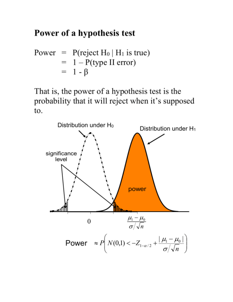
Power of a hypothesis test
Power = P(reject H0 | H1 is true)
= 1 – P(type II error)
= 1-β
That is, the power of a hypothesis test is the
probability that it will reject when it’s supposed
to.
Distribution under H0
Distribution under H1
significance
level
power

Power
1   0
 n

|   0 | 

 P N (0,1)   Z1 / 2  1
 n 

Example: Post-hoc power calc for Gum study
For the group-A gum data our test did not reject the null
hypothesis of no mean change in DMFS.

WE KNOW: our test does not furnish us good
evidence of a change in DMFS.

WE DON’T KNOW: Whether or not the DMFS truly
changes because the lack of evidence could be the
result of either:
a. the mean DMFS truly doesn’t change, or
b. the test wasn’t powerful enough to provide
evidence of change.
We can assess b. by estimating the power of our test.
WE KNOW: n=25, =0.05
ASSUME:
 true average change in the population is 1 DMFS
 true population standard deviation is σ=5.37.

|1 0 | 
  P( Z  1.03)  P( Z  1.03)  .152
P N (0,1)  1.96 
5.37 25 

Only 15% power. This implies the truth could be a. or b.
Example: Post-hoc power calc (continued)
Suppose now that we had seen the same result (did
not reject null hypothesis of no mean change), but the
sample size had been n=250.
The power from this hypothesis test would have
been:

|1 0 | 
  P( Z  0.98)  .836
P N (0,1)  1.96 

5
.
37
250


This says that if there truly were a change in dmfs of
1 or greater, our test probably (83.6% chance) would
have rejected the null hypothesis.
This yields more evidence for us to “accept” the null
hypothesis.
Important Point:
Ensuring reasonably high power of your test will
not only increase your chance of rejecting null
hypothesis, it will also facilitate interpretation of
your result should your test fail to reject.
Factors that affect the power of a test for 

Distribution under H0
Distribution under H1
significance
level
power
1   0
 n
0
Power

| 1  0 | 


 P N (0,1)   Z1 / 2 
 n 

 Power ↑as |μ0- μ1| ↑
 Power ↑as n ↑
 Power ↑as σ ↓
 Power ↑as α ↑
Sample Size Calculation
We can invert the power formula to find the
minimum n that will give a specified power.
To have power 1- β to reject for a test with
significance level  to reject the null hypothesis
H0: μ = μ0, in favor of H1: μ ≠ μ0 then the sample
size should be at least
 2 Z1 / 2  Z1  2
n
1  0 2
Example:
In our previous example, to have 80% power to
detect a difference of 1 DMFS, the sample size
should be at least
5.37 2 1.960  0.842 
n
 226.4 ,
2
1  0
2
so should enroll 227 kids.
To have 80% power to find a difference of 2 DMFS,
the sample size should be
5.37 2 1.960  0.842 
n
 56.6 .
2  02
2
Components in to a sample-size calculation
1. the desired power 1- β
2. the significance level α
3. the population standard deviation σ
4. the difference in the means |μ0- μ1|
1. The desired power 1- β:
Common “industry standard” is minimum 80%.
Tests attempting to demonstrate evidence of
equality (instead of differences) will sometimes
specify higher powers (95%)
2. Significance level α:
Usual choices are α = 0.05 or α = 0.01.
Sometimes adjustments for multiple testing will
lead to specifying other levels for α.
3. Population standard deviation σ:
The population standard deviation will not be
known, and must be estimated from previous
studies. These estimates should be conservative
(err on the high side).
Example: gum data
We estimated σ using s from a sample of size
n=25. The 95% confidence interval for σ in this
case would be (4.19, 7.47)*, so we see using σ =
5.37 may be an underestimate of the true
population SD.
Suppose we assumed σ = 5.37, so used a sample of
227 in hopes to have 80% power to detect a
difference of 1 dmfs. BUT, say that σ really was
6.00. Then our true power would be only

|1 0 | 
  P( Z  0.55)  .709 .
P N (0,1)  1.96 
6.00 227 

A conservative method is to use the upper 80%
confidence limit for σ, as an estimate for σ, which
2
2
is given by (n  1)s  n1,0.20 *.
*
see Rosner, section 6.7 for details of calculation
4. Difference in the means |μ0- μ1|
Specifying the alternative hypothesis mean is the
most tricky part of the calculation, and the choice
can greatly affect the power estimates (and thus
sample-size estimates).
60%
40%
0%
20%
power
80% 100%
power: n=57, sigma=5.37, alpha=0.05
0.0
0.5
1.0
1.5
2.0
2.5
3.0
true mean difference
Ideally one should specify μ1 to be the minimal
clinically significant difference.
Your study will have reasonable power to find a
difference of the size you specify in μ1. However, if
the true μ is smaller than μ1 your study has a good
chance of not rejecting H0. Thus you’d like μ1 to
specify the smallest difference you would consider an
interesting finding.