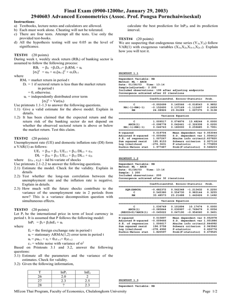
Final Exam (0900-1200hr, January 29, 2003)
2940603 Advanced Econometrics (Assoc. Prof. Pongsa Pornchaiwiseskul)
Instructions:
a) Textbooks, lecture notes and calculators are allowed.
b) Each must work alone. Cheating will not be tolerated.
c) There are four tests. Attempt all the tests. Use only the
provided test-books.
d) All the hypothesis testing will use 0.05 as the level of
significance.
TEST#1 (20 points)
During week t, weekly stock return (RB t) of banking sector is
assumed to follow the following process:
RBt = 0 +1Dt-1+2RMt + ut
[t]2 = 0 + 1[ut-1]2 + 2Dt-1
where
RMt = market return in period t
Dt = 1 if sectoral return is less than the market return
in period t
= 0, otherwise.
ut = independently distributed error term
[t]2 = Var(ut)
Use printouts 1.1-1.3 to answer the following questions.
1.1) Give a valid estimate for the above model. Explain in
details.
1.2) It has been claimed that the expected return and the
return risk of the banking sector do not depend on
whether the observed sectoral return is above or below
the market return. Test this claim.
TEST#2 (20 points)
Unemployment rate (UE) and domestic inflation rate (DI) form
a VAR(1) as follows:
UEt = 10 + 11 UEt-1 + 12 DIt-1 + 1t
DIt = 20 + 21 UEt-1 + 22 DIt-1 + 2t
where (1t , 2t) ~ iid bi-variate of shocks
Use printouts 2.1-2.2 to answer the following questions.
2.1) Estimate the model. Check for the validity. Explain in
details
2.2) Test whether the long-run correlation between the
unemployment rate and the inflation rate is negative.
Explain in details.
2.3) How much will the future shocks contribute to the
variance of the unemployment rate in 2 periods from
now? This is a variance decomposition question with
simultaneous effects.
TEST#3 (20 points)
Let Pt be the international price in term of local currency in
period t. It is assumed that P follows the following model:
lnPt = 1+ 2lnEt + ut
where
Et = the foreign exchange rate in period t
ut = stationary ARMA(1,2) error term in period t
ut = ut-1 + t + 1 t-1+ 2 t-2
 t = white noise with variance of 2
Based on Printouts 3.1 and 3.2, answer the following
questions:
3.1) Estimate all the parameters and the variance of the
estimates. Check for validity.
3.2) Given the following information,
T
26
27
28
lnPt
2.0
2.3
?
lnEt
2
2.5
2.3
calculate the best prediction for lnP28 and its prediction
interval.
TEST#4 (20 points)
We are suspecting that endogenous time series (Y1t,Y2t) follow
VAR(1) with exogenous variables (X1t,X2t,X1t-1,X2t-1). Explain
how you will test it.
PRINTOUT 1.1
============================================================
Dependent Variable: RB
Method: ML - ARCH
Date: 01/28/03
Time: 13:14
Sample(adjusted): 2 200
Included observations: 199 after adjusting endpoints
Convergence achieved after 22 iterations
============================================================
CoefficientStd. Errorz-Statistic Prob.
============================================================
C
-0.002699
0.145566 -0.018543
0.9852
RB(-1)<RM(-1)
-0.152600
0.137169 -1.112497
0.2659
RM
24.08926
23.91289
1.007375
0.3138
============================================================
Variance Equation
============================================================
C
1.009517
0.074876
13.48244
0.0000
ARCH(1)
-0.098778
0.042461 -2.326308
0.0200
RB(-1)<RM(-1)
0.046743
0.180000
0.259685
0.7951
============================================================
R-squared
0.019704
Mean dependent var 0.053044
Adjusted R-squared -0.005692
S.D. dependent var 1.004412
S.E. of regression
1.007267
Akaike info criteri2.837820
Sum squared resid
195.8153
Schwarz criterion 2.937116
Log likelihood
-276.3631
F-statistic
0.775859
Durbin-Watson stat
1.977487
Prob(F-statistic) 0.568203
============================================================
PRINTOUT 1.2
============================================================
Dependent Variable: RB
Method: ML - ARCH
Date: 01/28/03
Time: 13:16
Sample: 1 200
Included observations: 200
Convergence achieved after 32 iterations
============================================================
CoefficientStd. Errorz-Statistic Prob.
============================================================
SQR(GARCH)
-0.682372
0.562348 -1.213432
0.2250
C
0.545380
0.554730
0.983144
0.3255
RM
33.48573
23.21488
1.442426
0.1492
============================================================
Variance Equation
============================================================
C
1.036749
0.101894
10.17474
0.0000
ARCH(1)
-0.085844
0.030997 -2.769479
0.0056
(RESID<0)*ARCH(1) -0.045022
0.047190 -0.954060
0.3401
============================================================
R-squared
0.015897
Mean dependent var 0.052978
Adjusted R-squared -0.009466
S.D. dependent var 1.001886
S.E. of regression
1.006617
Akaike info criteri2.844992
Sum squared resid
196.5758
Schwarz criterion 2.943942
Log likelihood
-278.4992
F-statistic
0.626776
Durbin-Watson stat
1.820597
Prob(F-statistic) 0.679525
============================================================
PRINTOUT 1.3
============================================================
Dependent Variable: RB
MEcon Thai Program, Faculty of Economics, Chulalongkorn University
Page 1/2
Final Exam (0900-1200hr, January 29, 2003)
2940603 Advanced Econometrics (Assoc. Prof. Pongsa Pornchaiwiseskul)
Method: ML - ARCH
Date: 01/29/03
Time: 13:16
Sample: 1 200
Included observations: 200
Convergence achieved after 26 iterations
============================================================
CoefficientStd. Errorz-Statistic Prob.
============================================================
C
-0.033348
0.138380 -0.240988
0.8096
RM
22.53198
23.51115
0.958353
0.3379
============================================================
Variance Equation
============================================================
C
1.037565
0.102964
10.07699
0.0000
ARCH(1)
-0.098655
0.010456 -9.435508
0.0000
============================================================
R-squared
0.007892
Mean dependent var 0.052978
Adjusted R-squared -0.007293
S.D. dependent var 1.001886
S.E. of regression
1.005533
Akaike info criteri2.839077
Sum squared resid
198.1748
Schwarz criterion 2.905044
Log likelihood
-279.9077
F-statistic
0.519739
Durbin-Watson stat
1.861711
Prob(F-statistic) 0.669179
============================================================
Lags interval: 1 to 1
============================================================
Likelihood
5 Percent
1 Percent Hypothesized
Eigenvalue
Ratio
Critical ValuCritical ValuNo. of CE(s)
============================================================
0.389833
34.99342
15.41
20.04
None
0.103549
6.340073
3.76
6.65
At most 1
============================================================
*(**) denotes rejection of the hypothesis at 5%(1%)
significance level
Unnormalized Cointegrating Coefficients:
============================================================
UE
DI
0.075458
0.138147
0.090885
-0.039561
============================================================
PRINTOUT 2.1
Vector Autoregression Estimates
========================================
Date: 01/28/03
Time: 13:22
Sample(adjusted): 2 60
Included observations: 59 after adjusting
endpoints
Standard errors & t-statistics in parentheses
========================================
UE
DI
========================================
UE(-1)
0.484077
-0.186778
(0.10345)
(0.08903)
(4.67931) (-2.09803)
Log likelihood-165.0593
============================================================
DI(-1)
-0.312070
(0.10708)
(-2.91425)
0.335431
(0.09215)
(3.63996)
C
0.542541
0.227590
(0.18083)
(0.15561)
(3.00031)
(1.46253)
========================================
R-squared
0.382675
0.263981
Adj. R-squared
0.360627
0.237694
Sum sq. resids
67.11876
49.70590
S.E. equation
1.094783
0.942128
F-statistic
17.35697
10.04248
Log likelihood -87.52069
-78.66066
Akaike AIC
3.068498
2.768158
Schwarz SC
3.174136
2.873796
Mean dependent
0.973097
0.106559
S.D. dependent
1.369150
1.079059
========================================
Determinant Residual Covaria 0.950494
Log Likelihood
-165.9369
Akaike Information Criteria 5.828370
Schwarz Criteria
6.039645
========================================
Normalized Cointegrating Coefficients: 1 Cointegrating
Equation(s)
============================================================
UE
DI
C
1.000000
1.830790
-1.172253
(0.44837)
PRINTOUT 3.1
============================================================
Dependent Variable: LOG(P)
Method: Least Squares
Date: 01/28/03
Time: 13:39
Sample(adjusted): 2 27
Included observations: 26 after adjusting endpoints
Convergence achieved after 19 iterations
Backcast: 0 1
============================================================
Variable
CoefficientStd. Errort-Statistic Prob.
============================================================
C
0.556897
0.167547
3.323828
0.0032
LOG(E)
-0.404976
0.073326 -5.522935
0.0000
AR(1)
0.578664
0.301539
1.919035
0.0687
MA(1)
-0.977222
0.497775 -1.963178
0.0630
MA(2)
-0.011509
0.362611 -0.031740
0.9750
============================================================
R-squared
0.637016
Mean dependent var 0.423882
Adjusted R-squared
0.567876
S.D. dependent var 0.283021
S.E. of regression
0.186047
Akaike info criter-0.354592
Sum squared resid
0.726884
Schwarz criterion -0.112650
Log likelihood
9.609693
F-statistic
9.213453
Durbin-Watson stat
2.015074
Prob(F-statistic) 0.000184
============================================================
Inverted AR Roots
.58
Inverted MA Roots
.99
-.01
============================================================
PRINTOUT 3.2
Coefficient Covariance Matrix
============================================================
C
LOG(E)
AR(1)
MA(1)
MA(2)
============================================================
C
0.028072 -3.90E-05
0.030094 -0.064432
0.033179
LOG(E) -3.90E-05
0.005377 -0.000615 -0.005995
0.003812
AR(1)
0.030094 -0.000615
0.090926 -0.134770
0.099009
MA(1) -0.064432 -0.005995 -0.134770
0.247780 -0.171672
MA(2)
0.033179
0.003812
0.099009 -0.171672
0.131487
============================================================
End of Exam
PRINTOUT 2.2
Johansen Cointegration Test
============================================================
Date: 01/28/03
Time: 13:28
Sample: 1 60
Included observations: 58
Test assumption: Linear deterministic trend in the data
Series: UE DI
MEcon Thai Program, Faculty of Economics, Chulalongkorn University
Page 2/2