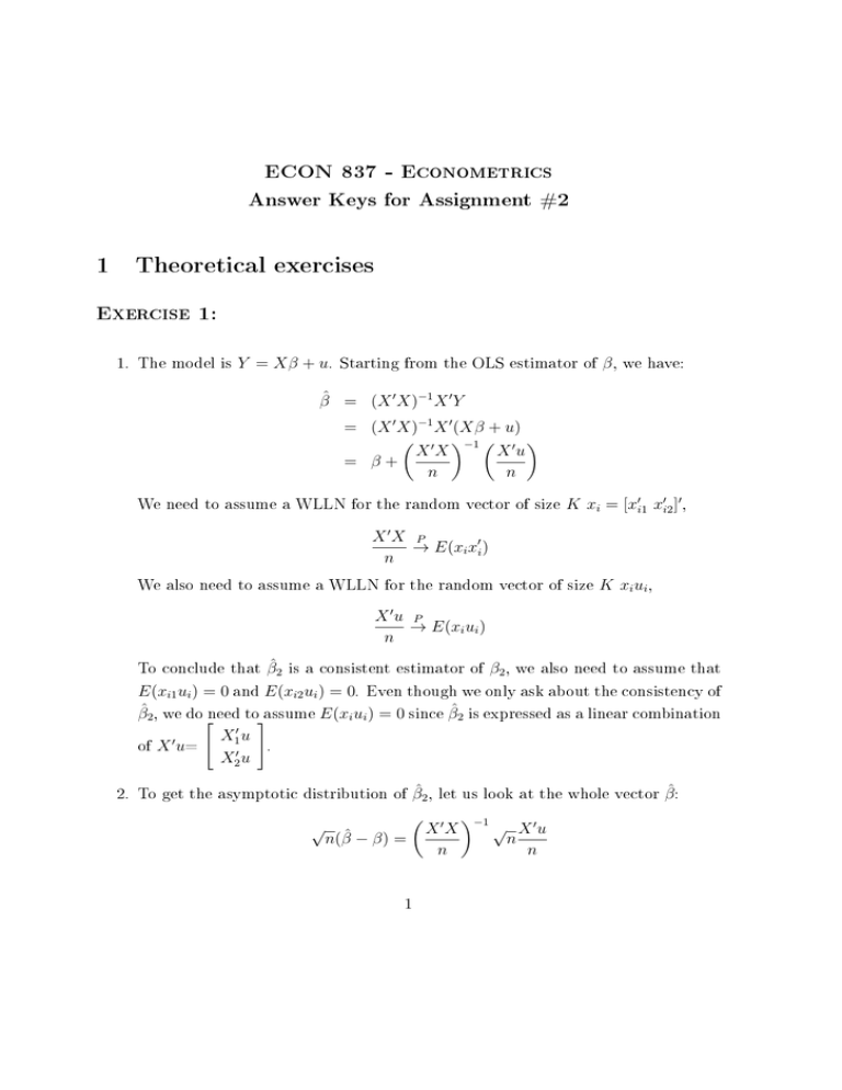
ECON 837 - Econometrics
Answer Keys for Assignment #2
1 Theoretical exercises
Exercise 1:
1. The model is Y = Xβ + u. Starting from the OLS estimator of β , we have:
β̂ = (X ′ X)−1 X ′ Y
= (X ′ X)−1 X ′ (Xβ + u)
( ′ )−1 ( ′ )
Xu
XX
= β+
n
n
We need to assume a WLLN for the random vector of size K xi = [x′i1 x′i2 ]′ ,
X ′X P
→ E(xi x′i )
n
We also need to assume a WLLN for the random vector of size K xi ui ,
X ′u P
→ E(xi ui )
n
To conclude that β̂2 is a consistent estimator of β2 , we also need to assume that
E(xi1 ui ) = 0 and E(xi2 ui ) = 0. Even though we only ask about the consistency of
β̂2 , we do[need to]assume E(xi ui ) = 0 since β̂2 is expressed as a linear combination
of X ′ u=
X1′ u
.
X2′ u
2. To get the asymptotic distribution of β̂2 , let us look at the whole vector β̂ :
√
n(β̂ − β) =
(
1
X ′X
n
)−1
√ X ′u
n
n
√
e.g. the asymptotic distribution of n(β̂2 − β2 ) is a linear combination of the
√
√
asymptotic distribution of X1′ u/ n and X2′ u/ n, hence we need to assume a
√
(joint) CLT for X ′ u/ n, namely
X ′u d
√ → N (0, E(xi x′i u2i ))
n
Then, we can deduce the asymptotic distribution of β̂ :
√
n(β̂ − β) → N (0, [E(xi x′i )]−1 E(xi x′i u2i )[E(xi x′i )]−1 )
d
Now to derive the asymptotic distribution of β̂2 , we need to nd the south-east
block of the asymptotic variance-covariance matrix of β̂ , which can be done (as
in assignment 1) by using the formula of the inverse of a block matrix.
3. The asymptotic variance-covariance matrix of β̂2 is called S2 , that is
√
d
n(β̂2 − β2 ) → Z2
with V ar(Z2 ) = S2 = AV ar(β̂2 )
The variance of β̂2 when the sample size is xed is
V ar(β̂2 ) = V ar([(X ′ X)−1 X ′ u]K2 ,K2 )
and we have
P
nV ar(β̂2 ) → S2
In other words, for xed n, V ar(β̂2 ) is approximately S2 /n.
Exercise 2:
1. The OLS estimator of β1 is:



y1
1




 y2 
 2 



with X = 
 ..  , y =  .. 
.
.




yT
T

∑
tyt
β̂1 = (X ′ X)−1 X ′ y = ∑t 2
tt
2
Recall:
T
∑
t=1
T (T + 1)
t=
2
and
T
∑
t2 =
t=1
T (T + 1)(2T + 1)
6
Hence:
β̂1 = β1 +
∑
6
tut
T (T + 1)(2T + 1) t
∑
By assumption, ut are iid, hence a LLN applies: (
since |t/T | < 1, we conclude that:
ut )/T → E(ut ). In addition,
P
t
∑
∑
1
6
P E(ut )
P
tut →
and
tut → 0
(T + 1)(2T + 1) t
2
T (T + 1)(2T + 1) t
Finally, we get: β̂1 → β1 .
P
2. From 1., we have:
T
T
(
)
∑
6
3 ∑
3/2
β̂1 − β1 =
tut ⇔ T
tut + op (1)
β̂1 − β1 = 3/2
T (T + 1)(2T + 1) t=1
T
t=1
By assumption, ut are iid with mean 0 and variance σ 2 . In addition,
∑
∑
E(
tut ) =
t×0=0
t
t
∑
∑
T (T + 1)(2T + 1) 2
V ar(
tut ) =
t2 σ 2 =
σ
6
t
t
3 ∑
tut ) = 3σ 2
and V ar( 3/2
T
t
(
)
Hence a CLT applies, and we have: T 3/2 β̂1 − β1 → N (0, 3σ 2 ).
3
d
3. The OLS residuals are ût = yt − β̂1 t. The associated estimator of the variance is:
1∑ 2
û
T t t
1∑
=
(yt − β̂1 t)2
T t
1∑
=
[ut + (β1 − β̂1 )t]2
T t
1∑ 2
1∑ 2
2∑
=
ut + (β1 − β̂1 )2 ×
t + (β1 − β̂1 ) ×
tut
T t
T t
T t
σ̂ 2 =
We study the convergence of each term separately:
1∑ 2 P 2
u →σ
T t t
(β1 − β̂1 )2 ×
1∑ 2
(T + 1)(2T + 1)
t = (β1 − β̂1 )2 ×
T t
6
= [T (β1 − β̂1 )]2 ×
(T + 1)(2T + 1)
6T 2
P
→ 0
by using the asymptotic distribution found in 2.
(β1 − β̂1 ) ×
2∑
P
tut → 0
T t
by using results found in 1.
To conclude, we have: σ̂ 2 → σ 2 , which means that it is a consistent estimator of
the variance of ut .
P
4