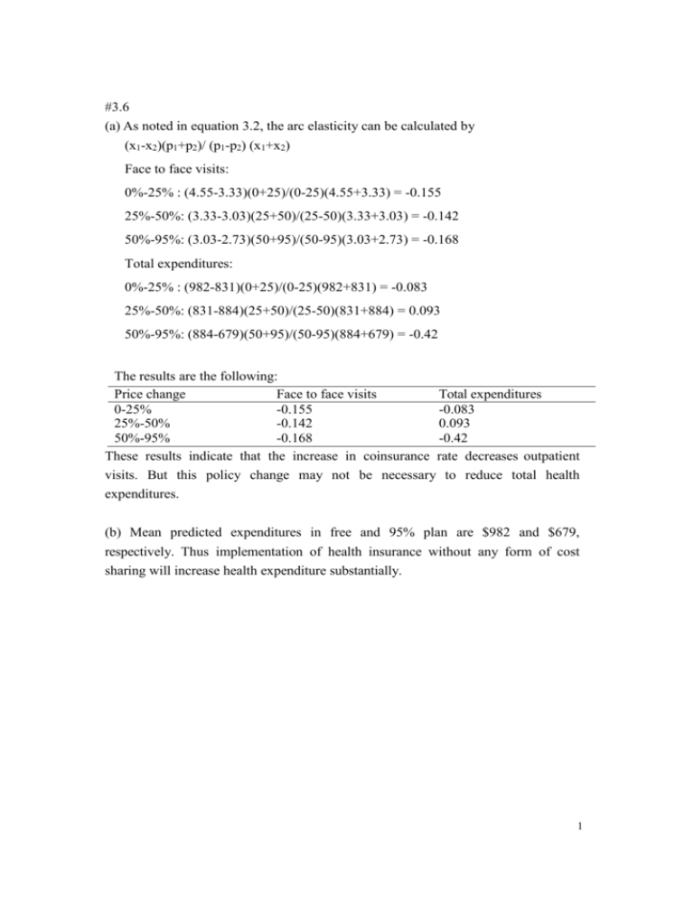
#3.6
(a) As noted in equation 3.2, the arc elasticity can be calculated by
(x1-x2)(p1+p2)/ (p1-p2) (x1+x2)
Face to face visits:
0%-25% : (4.55-3.33)(0+25)/(0-25)(4.55+3.33) = -0.155
25%-50%: (3.33-3.03)(25+50)/(25-50)(3.33+3.03) = -0.142
50%-95%: (3.03-2.73)(50+95)/(50-95)(3.03+2.73) = -0.168
Total expenditures:
0%-25% : (982-831)(0+25)/(0-25)(982+831) = -0.083
25%-50%: (831-884)(25+50)/(25-50)(831+884) = 0.093
50%-95%: (884-679)(50+95)/(50-95)(884+679) = -0.42
The results are the following:
Price change
Face to face visits
Total expenditures
0-25%
-0.155
-0.083
25%-50%
-0.142
0.093
50%-95%
-0.168
-0.42
These results indicate that the increase in coinsurance rate decreases outpatient
visits. But this policy change may not be necessary to reduce total health
expenditures.
(b) Mean predicted expenditures in free and 95% plan are $982 and $679,
respectively. Thus implementation of health insurance without any form of cost
sharing will increase health expenditure substantially.
1
(c) & (d) The individual deductible plan provides a mix of health insurance
coverage: For the smaller amount of health care expenditure, such as outpatient
expenditure, an insured individual needs to pay the cost by out-of-pocket payment.
Thus, the effect of individual deductible plan on the use of outpatient services is
similar to coinsurance plan. By contrast, for large amount of health care expenditure,
such as inpatient expenditure, the insurer pays the cost because the amount of
inpatient expenditure is more likely to exceed the threshold amount for deductibles.
Thus, the effect of individual deductible plan on the use of inpatient services is
similar to free plan.
#3.10
The following figure is used to answer the question:
p
E
Demand Curve
A
17
2
0
D
Old Plan
B
9
C
15
New Plan
x
The additional benefit from the six additional inhalers to Bill is the shaded area under
the demand curve between A and C, which is equal to 57 (= [(17- 2)×6]/2+2×6). The
six additional inhalers only cost Bill 12 (2×6). However, the insurer pays 90 (15×6)
for these six additional inhalers. Under the old plan, Bill’s consumer surplus is the
triangle represented by EA17. Under the new plan, Bill’s consumer surplus becomes
EC2. Thus, Bill is better off under the new plan.
17
#4.2
(a) Expected income (EY) = (0.4×2500)+(0.6×4900) = 3940
(b) Expected utility of income (EU) = 0.4×25000.5+0.6×49000.5 = 20+42 = 62 U[EY]
= 39400.5 = 62.77
(a) Since U[EY] > EU, John is a risk averter. John obtains a higher utility from a
certain income (3,940) than from two uncertain incomes. Thus, John prefers certain to
uncertain.
18
Utility (U)
U(4900)=70
U(EY)=62.7
EU=62
U(2500)=50
0
2500
Income (Y)
Y′ EY
4900
(3844)(3940)
(b) Given that U = Y0.5 and EU = 62, this implies Y′ = 3844.
The maximum amount that John is willing to pay to avoid the risk of income loss
= EY – Y′ = 3940 – 3844 = 96.
#4.3
The maximum amount that John is willing to pay to avoid the risk of income loss is
ww-ww′, where ww=wh-EL=(1-Θ)wh+Θws and ww′ is the wealth that satisfies the
condition that EU(w)=U(ww′). Based on the information given in exercise 4.2:
Probabilty
of
becoming
ww
ww′
ww-ww′
sick
Case 1
0.4
3,940
3,844
96
Case 2
0.5
3,700
3,600
100
John is more likely to buy health insurance in case 2 (probability of becoming sick is
0.4) than he would in case 1 (probability of becoming sick is 0.5) because the
maximum amount that John is willing to pay to avoid the risk of income loss is
higher in case 2 than in case 1.
19
#4.5
The actuarial value of the gamble is 100 (10,000 x 0.01). We can use the graph
shown in Fig. 4.4 to explain why the person would rather gamble than not gamble.
Since the individual is a risk lover, his or her marginal utility of wealth increases
with increases in wealth. This means that the expected utility of two uncertain
incomes (one is 10,000-the price of lottery, the other is 20,000) is higher than the
utility of certain income (10,000). Thus, the person is willing to pay more than 100
(expected gain) for having the opportunity to gamble.
20