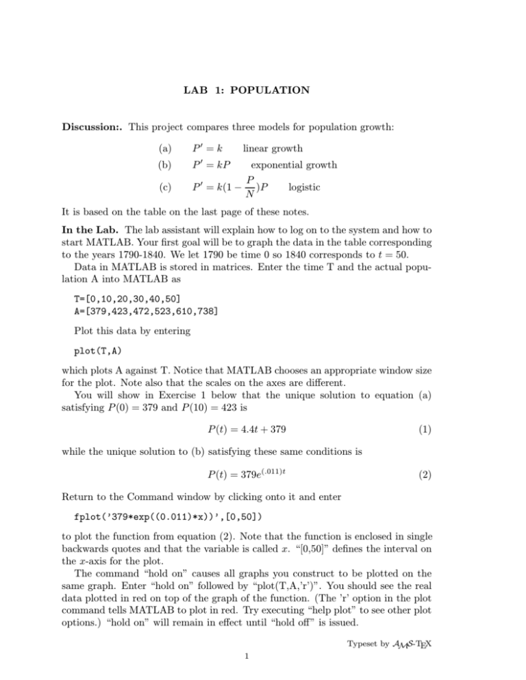
LAB 1: POPULATION
Discussion:. This project compares three models for population growth:
(a)
(b)
(c)
P0 = k
linear growth
0
P = kP
exponential growth
P
P 0 = k(1 − )P
logistic
N
It is based on the table on the last page of these notes.
In the Lab. The lab assistant will explain how to log on to the system and how to
start MATLAB. Your first goal will be to graph the data in the table corresponding
to the years 1790-1840. We let 1790 be time 0 so 1840 corresponds to t = 50.
Data in MATLAB is stored in matrices. Enter the time T and the actual population A into MATLAB as
T=[0,10,20,30,40,50]
A=[379,423,472,523,610,738]
Plot this data by entering
plot(T,A)
which plots A against T. Notice that MATLAB chooses an appropriate window size
for the plot. Note also that the scales on the axes are different.
You will show in Exercise 1 below that the unique solution to equation (a)
satisfying P (0) = 379 and P (10) = 423 is
P (t) = 4.4t + 379
(1)
while the unique solution to (b) satisfying these same conditions is
P (t) = 379e(.011)t
(2)
Return to the Command window by clicking onto it and enter
fplot(’379*exp((0.011)*x))’,[0,50])
to plot the function from equation (2). Note that the function is enclosed in single
backwards quotes and that the variable is called x. “[0,50]” defines the interval on
the x-axis for the plot.
The command “hold on” causes all graphs you construct to be plotted on the
same graph. Enter “hold on” followed by “plot(T,A,’r’)”. You should see the real
data plotted in red on top of the graph of the function. (The ’r’ option in the plot
command tells MATLAB to plot in red. Try executing “help plot” to see other plot
options.) “hold on” will remain in effect until “hold off” is issued.
Typeset by AMS-TEX
1
2
LAB 1: POPULATION
A few more useful commands are “cla”, which clears the Figure window and
“axis”, which sets the plotting range for x and y. For example, “axis([0,50,0,20])”
will force MATLAB to plot only the range 0 ≤ x ≤ 50 and 0 ≤ y ≤ 20. This is
useful when the scale chosen by MATLAB is so big that you cannot see the features
of interest.
Finally, a quick way of producing the vector T is with the command “T=0:10:50”.
Try it!
Assignment (Part 1).
By solving equations (a) and (b), verify formulas (1) and (2). Use these formulas
to predict the population in 2050. Graph the population predicted by formulas (1)
and (2) along with the actual population from 1790-1990. How much faith do you
have in your predictions?
If A = [a1 , a2 , . . . , an ] is a data vector and B = [b1 , b2 , . . . , bn ] is an approximation
to A, then one measure of the error in this approximation is
= |A − B| = |a1 − b1 | + |a2 − b2 | + · · · + |an − bn |
In MATLAB this is computed as
norm(A-B,1)
Compute for the approximations to the population from 1790-1990 obtained
from formulas (a) and (b) respectively. Do the computed values of support your
empirical observations? Explain.
Note: In MATLAB, if A is a vector, then, exp(A) is the vector obtained by applying the exponential function to each entry of A. Thus, the vector of predicted population values form formula (2) is describable in MATLAB as “379*exp((0.011)*T)”.
The vector from formula (1) admits a similar description.
Next find the solution to (b) that agrees with the given data at 1790 and 1980.
Plot this solution on a graph containing the actual data as well as the function
from formula (2). Which solution appears to more closely match the actual data?
Compute the corresponding values of . Do they agree with your observations? On
the basis of this information, what is your best guess for the population in 2050?
Use the closest year to 1930+seed*3 as t = 0 where “seed” is your personal seed
number which was assigned in lab class. Find the solution of (b) that agrees with
the actual data at T = 0 and T = 10. Discuss the accuracy of this approximation
both for t > 0 and t < 0. Use this model to predict the population in 2050.
Assignment (Part 2) (c).
The general (non-equilibrium) solution to (c) is
P (t) = N Aekt /(1 + Aekt )
where A is an arbitrary constant.
Approximate the values of k, A, and N where t = 0 is, once again, 1790. For
this, choose two values of time t1 and t2 that are not close to each other. Then
approximate P 0 (ti ) with
P 0 (ti ) ≈
P (ti + 10) − P (ti )
10
LAB 1: POPULATION
3
The equations
k
)P (t1 )2
N
k
P 0 (t2 ) = kP (t2 ) − ( )P (t2 )2
N
P 0 (t1 ) = kP (t1 ) − (
yield a system of two linear equations which can be solved to yield approximate
k
values for k and N
. Finally, solve the equation
P (0) = N A/(1 + A)
for A.
Plot this solution against the historical data and predict the population in 2000
and 2050.
Show that P = 0 and P = N are equilibrium solutions to (c). Draw (by hand)
a rough picture for the slope field for (c). You should find that if 0 < P (0) < N
then P (t) < N for all t and limt→∞ P (t) = N . Thus, N represents the maximum
population that the system can support. What, according to your work, will be the
maximum population of New York?
Your report. The body of your report should address the following issues, one
at a time, in the form of a short essay. In the process, you should also answer
the questions asked in the two parts of the lab. For each model, you must find
specific values for certain parameters (the growth-rate, carring capacity, etc.). Be
sure to give a complete justification for the choices you made. You should include
pictures and graphs of data as appropriate. (Remember that one picture is worth
a thousand words, but a thousand pictures aren’t worth anything.) The issues to
be addressed are:
(1) What differential equation was solved and how was the solution obtained?
Exactly how were the coefficients computed?
(2) What, according to each model, will the population in 2050 be? Which
prediction do you have the most confidence in. Why? Be sure discuss the
fit to the historical data (both recent and past) using both your graphs and
the values of .
(3) At what population level will New York stop growing? How confident are
you in this answer?
(4) What factors might cause your answers to deviate from the actual answers.
Specifically, what variables do your various models take into account and
what are some variables not accounted for.
The Population of New York (in thousands).
Year 1790 1800 1810 1820 1830 1840 1850 1860 1870 1880
Pop. 379 423 472 523 610 738 995 1231 1457 1783
Year 1890 1900 1910 1920 1930 1940 1950 1960 1970 1980 1990
Pop. 2239 2805 3366 3852 4250 4317 4691 5149 5689 5737 6016