10th European Simulation Symposium and Exhibition, Simulation in Industry, pp. 520-528, October 26-28, 1998, Nottingham, United Kingdom.
RESOURCE ALLOCATION AND SCHEDULING OF OPERATIONS IN
AN INTERMODAL TERMINAL
Marco Zaffalon, Andrea E. Rizzoli, Luca Maria Gambardella, Monaldo Mastrolilli
IDSIA – Istituto Dalle Molle di Studi sull’Intelligenza Artificiale
Lugano – Switzerland
E-mail: {zaffalon,andrea,luca,monaldo}@idsia.ch
KEYWORDS
Intermodal terminal simulation, flexible job-shop
scheduling, resource allocation, network flow
problem.
ABSTRACT
An approach to the problem of deciding which
equipment and manpower must be allocated over a
sequence of work shifts is presented. Once these
resources are given, a feasible and near-optimal
sequence of operations to load and unload a set of
ships harboured in an Intermodal Container
Terminal is found. The solution of the resource
allocation problem is based on a network design
formulation that assumes that the loading and
unloading processes can be modelled as a network
of container flows between the ships and the
terminal yard for all the work shifts. The solution
of the scheduling problem is thus fundamental to
ensure that these flows are sustained in each work
shift, by detailing for each container, the path to
follow from its origin to its destination. A discreteevent simulation model with a resolution down to
the single container unit is used to validate the
resource allocation and the scheduling policies.
INTRODUCTION
The management of an intermodal container
terminal is a complex process that involves a vast
number of decisions to be taken. Containers arrive
and leave on various transportation means such as
trucks, trains and vessels. An intermodal container
terminal plays a fundamental role in routing goods
to and from their origins and destinations. It is a
basic node in a transportation network, where
thousand of daily decisions are taken to manage
this sustained flow of containers.
The advent of management information services
and data processing greatly improved the ability of
terminal managers to control the whole process,
but yet raw data has to be analysed and treated to
provide some insight on the performance of
terminal operations. Simulation models and
Operations Research techniques have proven to be
a reliable and convenient tool to support the
decision-makers in the daily operations in many
cases (Hayuth et al. 1994, Blümel, 1997, Bruzzone
and Signorile, 1997).
Storing containers on the yard, allocating
resources in the terminal, and scheduling vessel
loading and unloading operations (L/U
operations, for brevity) are major problems in an
intermodal container terminal (Gambardella et al,
1998). In the last two years IDSIA has been
working on the case study of La Spezia Container
Terminal (LSCT), located in the Tyrrhenian Sea in
Italy.
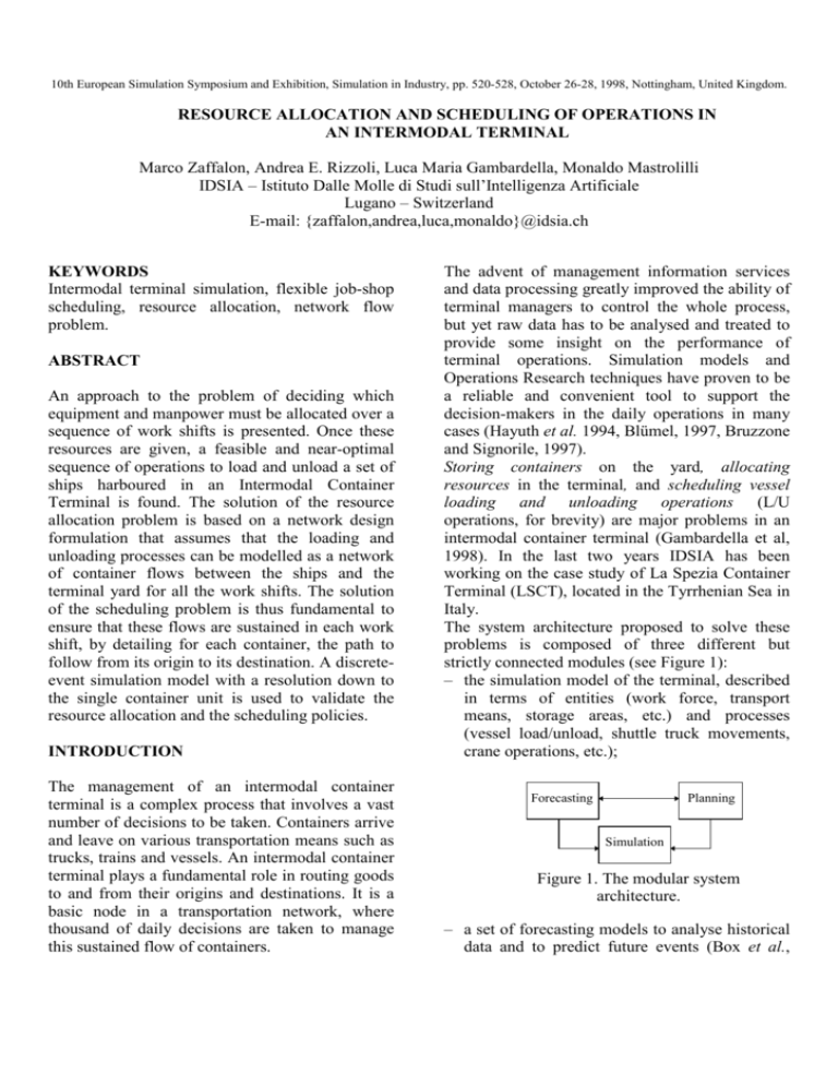
The system architecture proposed to solve these
problems is composed of three different but
strictly connected modules (see Figure 1):
– the simulation model of the terminal, described
in terms of entities (work force, transport
means, storage areas, etc.) and processes
(vessel load/unload, shuttle truck movements,
crane operations, etc.);
Forecasting
Planning
Simulation
Figure 1. The modular system
architecture.
– a set of forecasting models to analyse historical
data and to predict future events (Box et al.,
1994; Vemuri and Rogers, 1993), thus
providing estimates of the expected import and
export flows;
– the planning system which solves the problem
of the optimisation of L/U operations (L/U
problem), the problem of resource allocation
(RA problem), and the problem of the planning
and management of yard storage areas (space
problem).
This architecture supports the terminal managers
in the evaluation of:
– vessels loading and unloading sequences in
terms of time and costs;
– resource allocations procedures;
– policies for container storage both in terms of
space and cost of operations.
This allows terminal managers to assess “what-if”
scenarios; for instance, what happens if the
terminal undergoes an increased input/output
throughput, or even if structural changes are made
(e.g.: new berths are built, new cranes are added).
As the forecasting module is described in previous
papers (Gambardella et al., 1996, Bontempi et al.,
1997), in the following sections we introduce the
other two modules of our architecture: the planner
and the terminal simulator. In the planning module
the attention is focused on the problem of resource
allocation and scheduling of L/U operations, while
the planning and management of terminal yard
storage areas is out of the scope of the present
paper. For each topic, we present the major
problems, the resolution methodologies and the
experimental results obtained at the current state of
the project.
RESOURCE ALLOCATION
The LSCT is a terminal characterised by sustained
container traffic on a small yard area. The usual
state of the terminal is such that there are up to 4
large-sized ships, served in parallel by means of
(possibly) more than one quay crane each.
Containers for different ships share the space on
the yard, and as a consequence, yard resources
(gantry cranes, straddle cranes, fork lifters and
carts) are not pre-assigned to a ship, i.e. yard
resources are shared too. The role of the resource
allocation (RA) module is to determine the best
allocation of resources for vessel loading and
unloading operations, with the objective of
maximising the profit, given by the difference
between income and expenses (Zaffalon and
Gambardella, 1998). The income is a term
proportional to the number of moved container,
whereas the expenses are a linear function of the
allocated resources. Since more resources produce
a greater movement capacity, it is clear that the
RA problem corresponds to find the right balance
between moving containers while saving resource
costs. For what above, this can be achieved by
searching for the best way of sharing resources.
As far as RA is concerned, the terminal can be
interpreted as a mechanism which routes the
container flows from their sources to the proper
destinations. This view models the terminal as a
network of flow (Papadimitriou and Steiglitz,
10
15
Shift 1
CB1
CC1
30
45
CA1
QC1
Ship S1
R1
Shift 2
CA2
CB2
CC2
QC2
Ship S2
R2
Figure 2. The network flow problem over multiple
shifts.
1982). In such a network, the transport capacities
of the arcs are functions of the number of
resources that are allocated: hence, the focus is on
dimensioning arc capacities to maximise the profit.
The latter problem is a particular case of the socalled network design (Magnanti and Wong, 1984,
Ahuja et al., 1993). In the terminal case, the graph
of the network is also extended along the different
work shifts (1 shift = 6 hours) in order to represent
time (thus allowing the allocations to be computed
over all the period under study).
In Figure 2 we report a diagram showing a
graphical representation of an example problem.
Ship S is served by quay crane QC during a
sequence of shifts. The apex is used to denote the
current work shift, so that S1 is ship S served
during shift 1. L/U operations on S1 generate
different flows of container to and from the yard
storage areas where containers are to be picked up
or stored. In the example, the areas are CA, CB
and CC, served by gantry cranes (a type of yard
crane), and R, served by straddle cranes and fork
lifters, where 10, 15, 30 and 45 containers are
moved, respectively, during Shift 1. This implies
that QC during Shift 1 sustains a total flow of 100
containers. Thus, during the next shift, the total
number of containers to move is decreased by the
number of containers moved during the previous
shift (in our case 100). The problem is then to find
the best combination of quay cranes and yard
cranes to minimise the cost while balancing the
flow of containers to and from the ship over a
number of shifts which is limited by a deadline.
The resulting model is a complex mixed-integer
linear program, whose solution is demanded to the
branch & bound (Papadimitriou and Steiglitz,
1982) capabilities of Cplex 5 (Ilog, 1997). The
problem is solved in an approximate way, since
getting optimality is a time-consuming task in our
experience, because the complexity of the problem
produces a huge search tree. Notwithstanding, a
good solution is generally found quickly (few
minutes on a Pentium 133 MHz, 32 Mbytes of
RAM); experimental results based on real cases of
the LSCT show that the best integer value found is
usually close to the continuous bound.
SCHEDULING OF L/U OPERATIONS
The RA problem is necessarily a high-level
problem, since the resources must be allocated at
least 24 hours (up to a week) in advance, when the
data describing the ships and the yard state are
only partially known. When the ships arrive to the
terminal, the load/unload process is based on the
resources previously allocated and on the updated
state of the terminal. In particular, on the basis of
the latter information, the scheduling module must
build the Loading and Unloading List (LUL) for
all the ships at the terminal. The LUL is a
document that precisely specifies the origin and
the destination of every container to be moved to
and from the moored ships. As in the RA problem,
the focus is on the proper way of sharing resources
in order to produce a LUL that services the ships
within their (given) deadlines.
The difference with the RA problem is that
available resources are needed as input to the LUL
module. Hence, it does not take into account
economic factors, since the expenses are already
sustained at the time of the allocation of resources.
Rather, it must fill the gap between the two
different views of the terminal (high and lowlevel).
Our scheduling module is based on a Flexible JobShop (FJS) model, which is extended in order to
take into account set-up times of the resources and
to dynamically treat the evolution of the terminal.
It is heuristically solved by local search, according
to an original approach (Mastrolilli and
Gambardella, 1998). In the FJS problem n jobs are
processed to completion on a set of unrelated
machines. Each job consists of a sequence of
ordered operations where each operation has to be
executed on a machine out of a set of machines.
The processing time depends on the chosen
machine. Each machine is always available and it
is allowed to process one operation at a time
without preemption. The objective is to define the
operation sequence on each machine in order to
minimize the maximal completion time of all
operations (makespan).
When a ship arrives at the terminal, containers are
first unloaded from the ship, loaded on shuttle
trucks using the quay cranes and then stored on the
yard by the yard cranes. When the unloading
operations are finished, the loading stage can start:
containers are first fetched from the yard, loaded
on shuttle trucks using the yard cranes, then each
shuttle truck carries one container at a time to the
ship where it is loaded using a quay crane.
In our case a job is the sequence of loading and
unloading operations performed by a quay crane.
An operation is a container move. From an
analysis of the real world data, the yard cranes
appeared as the bottleneck machines for the
problem, thus suggesting to model them as
machines in a FJS based model. The goal is to
maximize their performances.
Hence, the problem is solved finding which yard
crane moves which container (routing problem)
and when (sequencing problem) in order to
minimise the maximum completion time of all
operations. The processing times of each machine
are assumed deterministic. We have tuned and
validated our model using real world data. Our
optimisation procedure is able to improve the yard
crane performances of about 31%. The
computational effort is very low, about 1 minute
on a 266 MHz Pentium for each shift. The latter
feature makes it possible to use the proposed
procedure as a reactive scheduler in order to
manage unexpected events.
In Figure 3 a sample output from the scheduling
module is reported. The yard cranes are listed on
the y-axis, while time (in seconds) on the x-axis.
Each box represents an operation (a container
move), its width is the time taken to complete the
operation. The numbers associated with each box
identify the quay crane that has performed that
operation.
SIMULATION
The simulator is used as a test bench to evaluate
the management policies produced by the
optimisation modules (Rizzoli et al., 1997). The
Figure 3. The Gannt chart is representing the solution
of the scheduling problem.
performances of various resource allocation
policies, used in conjunction with computer
generated L/U lists, are compared with real world
data. The indicator used to compare the solutions
is the net profit of the terminal operations during
the simulation horizon. This indicator takes into
account the cost of cranes and operators during the
various work shifts, the penalty to be paid to the
shipping company if the ship departure is delayed
and the income generated by each container loaded
and unloaded from a ship. Besides these
economical indicators, the simulator allows to
assess the resource utilisation and the measure
important congestion indicators such as the
average queue length of operations on the terminal
cranes.
Before assessing the validity of the resource and
L/U policies, the simulator must be calibrated and
validated in order to verify its capability of
reproducing the real terminal behaviour (Banks et
al. 1996).
The calibration and validation data were extracted
from a period of two weeks, from 5/11/1998 to
5/24/98. The data describe the activity of LSCT in
great detail, in such a way that every container
movement can be tracked down. In particular, the
database reports the resources that have moved a
container, the time that operation and the origin
and destination of the movement, identified by
bay, row and tier both on the ship and on the yard.
Furthermore, the database tracks the activity of
every transport mean that enters and leaves the
terminal (ships, trucks, trains). Notice that in the
calibration and validation phase, the simulation
module evolves using the same inputs and policies
used by the terminal management over the
calibration and validation periods. For this reason,
the resource allocation and the L/U policies are the
ones adopted by terminal managers during the
periods when calibration and validation data were
collected.
After performing a few screening experiments it
resulted that the simulation model was most
sensitive to changes in the parameters describing
the time required to move a container for a yard
and a quay crane and to a change in the time of
travel of a shuttle truck from the quay to the yard.
These parameters were modelled by normal
distributions. We recall that, during simulation,
ship, trains and truck arrivals are deterministic. We
are focusing our attention on a trace-driven
simulation for the purpose of generating a test
environment for the management policies.
In the simulation a grand total of 2950 containers
is moved over 10 work shifts. In order to find the
best combination of parameters among the
different experiments, the sum of the absolute
weighted errors over the examined work shifts for
each quay crane and yard crane is computed, as
given by the formulae below,
J qc =
J yc =
∑ ∑
qi , t − qi ,t
k
m
i =1
t =1
qmax
k
∑ ∑
h
m
i =1
t =1
yi ,t − yi ,t
y max
h
where i is the crane index and t is the work shift
index. The quantity qi,t represents the number of
simulated containers moved by quay crane i in the
t-th shift, while qi , t are the containers moved in the
real world, qmax and ymax represent the theoretical
maximum number of containers which can be
moved by a crane during one shift. There are h
yard cranes and k quay cranes. The formula for
yard cranes is similar, except for the aggregation
of single cranes in “macro-cranes”: for instance,
the two yard cranes working on area CB were
aggregated in a single yard crane, as it happened to
the fork lifts working on the areas served by
mobile carriers. Jqc and Jyc are therefore measures
of the simulation error, both for loading and
unloading. These errors are averaged over the
number of shifts and number of cranes.
After performing a set of experiments, we
obtained for the quay cranes an average calibration
error of 13.6% and a validation error of 14.2 %.
For the yard cranes, the results are slightly better,
6% in calibration and 13% in validation. These
results deserve a few words of comment, since
they seem susceptible to improvements. An
important remark is that our main objective is to
obtain a model of the terminal to test alternative
scheduling policies. For this purpose, the model,
as a first approximation, does not handle
unexpected and rare events such as crane
breakdowns, and inexperienced operators.
Unfortunately, such events happen in the real
world terminal, and this is evident, for instance, in
shift 1 on Q6, where the crane performance is well
below average, despite the terminal is working at
half capacity since this is a shift when trucks and
trains do not arrive. A more detailed analysis of
the real world data helps to discover that Q6
moves fewer containers than the average since it
stops working for some periods during the work
shift.
We are interested in designing a simulation model
that represents the “average” behaviour of the
terminal, where the only bottlenecks can be caused
by resource competitions on the yard, since we are
designing scheduling policies for a terminal where
the cranes are operating. Scheduling in front of
unexpected events, such as breakdowns, would be
the subject of a research into reactive scheduling
techniques.
INTERLEAVING THE MODULES
The problem of creating the L/U list is
hierarchically lower than RA (Gambardella et al.
1998). For this reason, it usually has a shorter time
horizon and a more detailed view of the terminal.
The L/U problem is mainly a scheduling problem.
Its input data are the allocated resources, the
container types, their amount and disposition both
on ships and at the terminal yard. For every quay
crane working on a ship at the terminal, the
module must output an order list of containers to
be loaded and unloaded. If the container is to load,
the list indicates the location in the ship where it
must be put; in the same way, it reports the final
destination on the yard for the unloading
containers.
In this context, the simulator acts by requiring the
resources to the RA module and the L/U policies
to the L/U list generator module when needed.
Then, it makes the terminal state evolve according
to the information above and to external events
(ship arrivals, train/trucks arrivals; the latter are
generated and distributed according to one of the
patterns studied by a forecasting module). The RA
policy and the L/U policy are then successful if the
simulation is able to carry out all the jobs for the
period under study. Also the robustness of the
policies can be checked; this is obtained by means
of repeated applications of the simulation above
(in fact, the replications are normally different
since the simulation is non-deterministic).
Figure 3 reports the interaction of the three
modules in our experiments: the RA module, the
‘
S im u la tio n T im e
C u r r e n t S ta te
R A ([D 3 , D 9 ])
D ay 2
L U L (IV )
IV
L /U li s t
S IM (IV )
Resources for Day 2
C o n ta i n e r s M o v e d
III
II
L U L (III)
L /U li s t
S IM (III)
C o n ta i n e r s M o v e d
L U L (II)
L /U lis t
S IM (II)
C o n ta in e rs M o v e d
I
L /U li s t
S IM (I)
C u rre n t S ta te
R A ([D 2 , D 8 ])
Resources for Day 1
D ay 1
L U L (I)
D ay 0
R A ([D 1 , D 7 ])
C u rre n t S ta te
Figure 4. Architecture of the simulationoptimisation phase.
L/U list generator module (LUL) and the simulator
(SIM). The vertical axis represents simulation
time. At the beginning of day 0, the RA module is
ran, having as input the predicted state of ships in
the period from day 1 to day 7. On its basis, the
module is able to compute the resources to use in
the same period (notice that RA must compute the
resources to allocate with one day in advance,
because this is the minimum span to book
resources). Notwithstanding, only the resources
computed for the first day (day 1) are used. The
reason is that the reliability of the prediction used
by RA quickly decreases with time. Therefore we
chose to let the RA module have a time window of
one week, while its output is used for the first day
only.
The output of the RA module (at day 0) is passed
as input to the box representing the interaction
between the LUL and SIM modules in a time
period of one day (notice that the day is split into
four shift of six hours each). They use the
allocated resources and the current state of the
terminal (in terms of ship and yard states). In
particular, at the first shift of day 1, the LUL
module produces the L/U list for the ships
currently at the terminal. Then the simulation tool
emulates the terminal for the current shift, having
as input the state of terminal, the allocated
resources and the L/U list.
At the end of the shift, the containers that have
really be moved (by the simulator) are passed back
to the LUL module in order to let it update its
knowledge of the terminal state. On this basis, the
LUL produces the list for the second shift, and so
on up to the last shift of day 1. At the end of day 1
the current state of the terminal is passed to the
RA module, which, also on the basis of the
prediction for days 2 to 9, produces the allocation
for day 3. The process is then repeated until the
end of the simulation-optimisation period.
COMPUTER GENERATED RA AND LUL
TO IMPROVE TERMINAL MANAGEMENT
We have performed the cyclic process of “allocate
schedule simulate” described in the previous
section in order to discover if the computer
generated management policies were feasible once
implemented in the low-detail simulation model.
Moreover, we were interested in discovering how
the terminal would have reacted to the
implementation of such policies, especially for
what it concerned the behaviour of the yard cranes.
The computer generated RA policies allowed an
average saving of 30%. This means that fewer
resources were used to perform the same tasks. It
is important to notice that the computer generated
RA does not impose a quay crane intensity
(number of container moved per hour) higher than
the one normally attained by the real world
terminal. The RA module uses the real world crane
intensities as a parameter to fix the arc capacities.
CONCLUSIONS AND FUTURE RESEARCH
Number of Operations
YC5 and YC6 in Simulation with real data
45
40
35
30
25
20
15
10
5
0
1
2
3
4
5
6
7
Sub Areas inside CB
Number of Operations
YC5 and YC6 with Optimized work
40
35
30
25
20
15
10
5
0
1
2
3
4
5
6
7
Sub Areas inside CB
Figure 6. Areas of activity of the yard cranes.
Queues on YC05 with optimization
queue length
5
4
3
2
1
43
40
37
34
31
28
25
22
19
16
13
7
10
4
1
0
container number
Queue on YC05 during simulation with real data
5
queue length
4
3
2
1
49
45
41
37
33
29
25
21
17
13
9
5
0
1
Since the improvement is not to be found in an
increase of the quay crane intensities, it is instead
due to a more rational use of night shifts (which
are more expensive) on one hand and by a better
organisation of the yard crane work on the other.
In fact, it turns out that optimised LUL allow a
more efficient use of yard cranes, thus increasing
their intensity. This is possible since the yard crane
“conflicts” (i.e. when two yard cranes try to access
two containers which are very close at the same
time) are dramatically reduced. The reason for the
reduction is shown in Figure 6: without
optimisation, yard cranes YC05 and YC06 tend to
cover the whole area CB, while, with optimisation,
YC05 covers only the left hand side of CB and
YC06 the right hand side, thus virtually
eliminating the possibility of conflicts.
Another desirable side effect of optimisation is the
average reduction of queue lengths under yard
cranes: a better balance in the crane usage reduces
the possibility of having lengthy queues, as it is
shown in Figure 5.
container number
Figure 5. Queues of containers under the yard
cranes.
This paper presents the part of our research work
aimed at improving the management practices of a
container terminal. Using a simulation model of
the terminal we evaluate policies generated by
optimisation algorithms. Here the simulator acts as
a test bench for assessing the effectiveness and the
robustness of the policies in such a nondeterministic environment.
Simulation results show that the application of
computer generated management policies could
improve the terminal performance, making
possible the allocation of fewer resources, thanks
to a better usage of the yard cranes.
We are currently working on the space allocation
module, which performs the task of allocating
container on the yard. A better organisation of the
storage areas can lead to improvements in resource
allocation and loading and unloading scheduling
policies.
The combined system (i.e., optimisation and
simulation), once tested, can be the main
component of a decision support system for
terminal management, where the port managers
can test and evaluate different strategies,
comparing their own choices with the computer
generated ones, then selecting the best suited for
the current situation.
ACKNOWLEDGEMENT
This research is supported by Swiss UFES project
97.0315 under the European Project PLATFORM.
REFERENCES
Ahuja, R., T. Magnanti, J. Orlin. 1993. Network Flows,
Prentice Hall, New Jersey.
Banks, J., J.S. Carson, B.L. Nelson. 1996. DiscreteEvent System Simulation, 2nd edition. Prentice Hall,
Upper Saddle River, New Jersey.
Blümel E. (ed.). 1997. Managing and Controlling
Growing Harbour Terminals. Society for Computer
Simulation International.
Bontempi, G., L.M. Gambardella, A.E. Rizzoli. 1997.
“Simulation and optimisation for management of
intermodal terminals.” In: Proceedings of the 1997
European Simulation Multiconference (Istanbul, Tr,
June 1-4). Society for Computer Simulation
International.
Box, G.E.P., G.M. Jenkins, G.C. Reinsel. 1994. Time
Series Analysis: Forecasting and Control. Prentice
Hall, London.
Bruzzone, A.G., R. Signorile. 1996. “Genetic
algorithms and simulation as support for planning a
th
port terminal.” In: Proceedings of the 8 European
Simulation Symposium (Genoa, I, 24-26 October).
Society for Computer Simulation International.
Gambardella, L.M., G. Bontempi, E. Taillard, D.
Romanengo, G. Raso, P. Piermari. 1996. “Simulation
and forecasting in intermodal container terminal.” In:
Proceedings of the 8th European Simulation Symposium
(Genoa, I, 24-26 October). Society for Computer
Simulation International.
Gambardella, L.M., A.E. Rizzoli, M. Zaffalon. 1998.
“Simulation and planning of an intermodal container
terminal.” Simulation, Special Issue on Harbour and
Maritime Simulation, no. 71, vol. 2: 107–116.
Hayuth, Y., M.A. Pollatschek, Y. Roll. 1994. “Building
a port simulator.” Simulation, no. 63, vol. 3: 179–189.
Ilog. 1997. Cplex 6 User’s Manual,
http://www.cplex.com
Magnanti, T.L., R.T. Wong. 1984. “Network design
and transportation planning: models and algorithms.”
Transportation Science, no. 18, vol. 1: 1–56.
Mastrolilli, M., L.M. Gambardella. 1998. “New
neighborhood function for the flexible job shop
problem.” Technical Report n. 5-98. IDSIA,
Lugano,CH.
Rizzoli, A.E., L.M. Gambardella, G. Bontempi. 1997.
“Simulation of an intermodal container terminal to
assist the management in the decision making process.”
In: Proceedings of MODSIM ’97 (Hobart, Tas. 8-11
December). The Modelling and Simulation Society of
Australia Inc.
Vemuri, V.R., R.D. Rogers, Artificial Neural
Networks: Forecasting Time Series (IEEE Computer
Society Press, 1993)
Zaffalon, M., L.M. Gambardella. 1998. “A network
design approach to the allocation of resources in an
intermodal terminal.” Technical Report n. 10-98.
IDSIA, Lugano, CH.
BIOGRAPHY
Marco Zaffalon received the cum laude "laurea"
degree in computer science from the Università
degli Studi di Milano (Italy) in 1991 and the Ph.D.
in applied mathematics from the same university
in 1997. His interests are in the area of uncertain
reasoning (Bayesian networks) and operations
research (combinatorial optimization). Since 1997
he works as a researcher at IDSIA, where his main
activity is related to intermodal transportation
problems.