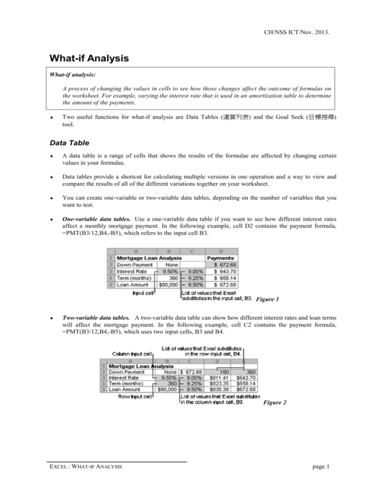
CH/NSS ICT/Nov. 2013.
What-if Analysis
What-if analysis:
A process of changing the values in cells to see how those changes affect the outcome of formulas on
the worksheet. For example, varying the interest rate that is used in an amortization table to determine
the amount of the payments.
♦
Two useful functions for what-if analysis are Data Tables (運算列表) and the Goal Seek (目標搜尋)
tool.
Data Table
♦
A data table is a range of cells that shows the results of the formulae are affected by changing certain
values in your formulas.
♦
Data tables provide a shortcut for calculating multiple versions in one operation and a way to view and
compare the results of all of the different variations together on your worksheet.
♦
You can create one-variable or two-variable data tables, depending on the number of variables that you
want to test.
♦
One-variable data tables. Use a one-variable data table if you want to see how different interest rates
affect a monthly mortgage payment. In the following example, cell D2 contains the payment formula,
=PMT(B3/12,B4,-B5), which refers to the input cell B3.
Figure 1
♦
Two-variable data tables. A two-variable data table can show how different interest rates and loan terms
will affect the mortgage payment. In the following example, cell C2 contains the payment formula,
=PMT(B3/12,B4,-B5), which uses two input cells, B3 and B4.
Figure 2
EXCEL : WHAT-IF ANALYSIS
page 1
CH/NSS ICT/Nov. 2013.
♦
Steps to create a one-variable data table
You must design one-variable data tables so that input values are listed either down a column (columnoriented) or across a row (row-oriented). Formulas that are used in a one-variable data table must refer to
an input cells.
i.
Type the list of values that you want to substitute in the input cell either down one column or across
one row.
ii.
Do one of the following:
a.
If the data table is column-oriented, type the formula in the row above the first value and one
cell to the right of the column of values (D2 in figure 1). Type any additional formulas to the
right of the first formula.
b.
If the data table is row-oriented, type the formula in the column to the left of the first value and
one cell below the row of values. Type any additional formulas below the first formula.
iii.
Select the range of cells that contains the formulas and values that you want to substitute.
iv.
On the Data tab, in the Data Tools group, click What-If Analysis, and then click Data Table.
Cell reference of the
input for a columnoriented data table
v.
♦
Do one of the following:
a.
If the data table is column-oriented, type the cell reference for the input cell in the Column
input cell box.
b.
If the data table is row-oriented, type the cell reference for the input cell in the Row input cell
box.
Create a two-variable data table
Two-variable data tables use only one formula with two lists of input values. The formula must refer to
two different input cells.
i.
In a cell on the worksheet, enter the formula that refers to the two input cells.
ii.
In figure 2, where the formula's starting values are entered in cells B3, B4, and B5, you would type
the formula =PMT(B3/12,B4,-B5) into cell C2.
iii.
Type one list of input values in the same column, below the formula.
iv.
In figure 2, you would type the different interest rates into cells C3, C4, and C5.
v.
Type the second list in the same row, to the right of the formula.
vi.
In figure 2, you would type the loan terms (in months) into cells D2 and E2.
vii.
Select the range of cells that contains the formula and both the row and column of values.
viii.
In figure 2, you would select the range C2:E5.
EXCEL : WHAT-IF ANALYSIS
page 2
CH/NSS ICT/Nov. 2013.
ix.
On the Data tab, in the Data Tools group, click What-If Analysis, and then click Data Table.
x.
In the Row input cell box, enter the reference to the input cell for the input values in the row.
xi.
In the example, you would type cell B4 in the Row input cell box.
xii.
In the Column input cell box, enter the reference to the input cell for the input values in the column.
xiii.
In the example, you would type B3 in the Column input cell box.
xiv.
Click OK.
Goal Seek 目標搜尋
♦
In Microsoft Excel, you can use the Goal Seek(目標搜尋) command (on the Tools 工具 menu) when you
know the result you want to return a formula, but you do not know the input values the formula needs to
reach that result. When you use goal seeking, Microsoft Excel varies the value in a specified cell until the
formula that is dependent on that cell returns a specified result.
♦
In the Goal Seek dialog box, you specify the cell containing the formula (Set Cell), the result you want
the formula to return (To Value) and one of the cells that the formula is dependent on (By Changing
Cell). Both of the cell specifications must be a single cell reference or name. The To Value must be a
number.
♦
In the following example, the value in B16 will be adjusted so as to get the result in H15 to be 1500
♦
EXCEL : WHAT-IF ANALYSIS
page 3