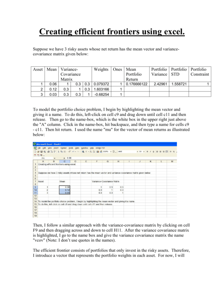
Creating efficient frontiers using excel.
Suppose we have 3 risky assets whose net return has the mean vector and variancecovariance matrix given below:
Asset Mean VarianceCovariance
Matrix
1
2
3
0.06
0.12
0.03
1
0.3
0.3
0.3
1
0.3
Weights
0.3
0.3
1
0.079372
1.603166
-0.68254
Ones Mean
Portfolio
Return
1
1
1
0.176666122
Portfolio Portfolio Portfolio
Variance STD
Constraint
2.42961
1.558721
To model the portfolio choice problem, I begin by highlighting the mean vector and
giving it a name. To do this, left-click on cell c9 and drag down until cell c11 and then
release. Then go to the name-box, which is the white box in the upper right just above
the "A" column. Click in the name-box, hit backspace, and then type a name for cells c9
- c11. Then hit return. I used the name "mu" for the vector of mean returns as illustrated
below:
Then, I follow a similar approach with the variance-covariance matrix by clicking on cell
F9 and then dragging across and down to cell H11. After the variance covariance matrix
is highlighted, I go to the name box and give the variance covariance matrix the name
"vcov" (Note: I don’t use quotes in the names).
The efficient frontier consists of portfolios that only invest in the risky assets. Therefore,
I introduce a vector that represents the portfolio weights in each asset. For now, I will
1
assign the weights arbitrarily. Below, I will use excel to choose the weights optimally.
For now, I have placed the weights in cells J9 through J11 and given them the name
weights. Also, for convenience, I have created a column of ones and given it the name
ones.
To illustrate why the names are convenient, note that for given portfolio weights, the
mean return on the risky asset portfolio is equal to the transpose of the weights vector
multiplied by the mean vector. Using excel's matrix formula's, the transpose of the
weights vector is given by "transpose(weights)", and to multiply "transpose(weights)" by
the mean vector "mu" simply requires using the excel function mmult, which stands for
matrix multiplication. The resulting mean return for the portfolio is given by
mmult(transpose(weights),ones). In this expression, excel multiplies the transpose of
weights by the vector of ones, producing the mean return on the portfolio.
To program the mean return and store it in a cell, one uses the excel format for matrix
formulas. For example, to store the mean return for the given weight vector in cell N9,
click on cell N9, and then type "= mmult(transpose(weights),mu)" and then hit CTRL
SHIFT ENTER. The quantity in the cell will be equal to the mean return and will change
when the weights change or when the elements of the mean return vector change.
To program the variance of the portfolio return, I use the fact that the variance of the
portfolio return is the transpose of the weights vector multiplied by variance covariance
matrix multiplied by the weights vector. To program this, first I multiply the transpose of
of weights vector times the variance-covariance matrix. This produces the expression
mmult(transpose(weights),vcov). Then, I have to multiply this expression by weights.
Therefore, the final answer for portfolio variance is
mmult(mmult(transpose(weights),vcov),weights). I have typed this expression into cell
O9 using the same approach that I used for typing the mean return. Clicking on the cell
will highlight the formula at the top of the excel spreadsheet. By changing the weights or
changing the elements of the variance covariance matrix, the portfolio variance will
change. The standard deviation of the portfolio return is just the square-root of the
variance, and is given in cell P9. To compute portfolio std, I named portfolio variance
portvar. The formula for portfolio std (standard deviation) is just portvar^.5. It is entered
in cell P9 with an equal sign before the formula. Then you hit return to enter the formula.
We are almost ready to start to use excel to compute the efficient frontier for this set of 3
assets. To compute the efficient frontier, we need to constrain the portfolio weights so
that that they sum to 1. This is equivalent to imposing the condition that
mmult(transpose(ones),weights) sums to 1. We will impose this constraint when choosing
portfolio weights. To do so, I have assigned the constraint to cell N17 by typing the
formula mmult(transpose(ones),weights) into the cell. When I use the constrained
maximization program, I will set the cell equal to 1, which will constrain the weights that
I can choose. I have chosen to name the constraint "constraint".
The last item to note before beginning to use solver is that it is useful to store the results
of maximization problems in a convenient form for further analysis. Towards this end, in
row 79 I have stored the weights vector along with mean portfolio return and portfolio
std. To illustrate how this was done, I highlighted cells b79-d79 and then in the formula
bar typed =transpose(weights) and hit CTRL SHIFT ENTER. This puts the transpose of
the weights in a 1 by 3 row vector. Then, in cells e79, f79, and g79, I simply repeated the
names portmean,, portvar, and portstd. This produces the same values at these cells that
were computed earlier.
weights
0.079372 1.603166 -0.68254
mean
variance std
0.176666 2.42961 1.558721
USING SOLVER TO FIND PORTFOLIO WEIGHTS
The textbook provides the answer to solving for the efficient frontier when there are 2
risky assets. When there are more than two risky assets, there are more complicated
matrix formulas for solving for the efficient frontier. If there are complicated constraints,
there may not be a formula for the efficient frontier. In this course, I will emphasize
using a maximization program to solve for the efficient frontier. More specifically, we
will use the excel program SOLVER to find the points on the efficient frontier.
SOLVER is an excel add-in package. To find solver, click on tools on the menu bar. If
you see solver in the menu, then it is installed and ready to be used. If you don't find
solver, then click on tools, Add-Ins, then check Solver, and click OK. This should give
you the capability to use solver.
To illustrate how to use to find points on the efficient frontier, recall that the lowest point
on the efficient frontier is the point that minimizes standard deviation of the portfolio
return. To solve for the mean and std of return of the minimum std portfolio, and to solve
for the weights in the portfolio, click on cell h79 (with the std on top) and then click on
tools, solver. The result should give you a window that appears as follows:
Click on set target cell, then, if it not already highlighted, click on h79 because we want
to minimize portfolio std. After choosing the target cell then click on Min because we
want to minimize the value of portfolio standard deviation. To do this, we change the
weights in the portfolio, hence, write in weights where it says by changing cells. Then,
where it says subject to the constraints click Add. This should bring up a window for
each constraint. The window will appear as follows:
For cell reference, fill in constraint (the name of the constraint). Click on the arrow and
choose equal. Then in the box that says constraint, fill in the number 1. This constraint
entered in this way guarantees that the weights sum to 1. Then click OK if this is the last
constraint that has been added.
After you have filled in all of the appropriate information in the solver box, it should
appear as follows.
Then, clicking Solve allows solver to choice the optimal portfolio weights to solve this
problem.
The weights, mean return, and standard deviation in line 79 will have changed because I
used solver. In particular, the new weights are those associated with the minimum std
portfolio. The same is true of the mean, variance, and std of the portfolio.
To save the new results, highlight them with your cursor, then right click and choose
copy. Then, highlight the part of a row with the same number of elements where you
want you save your results, and then right click and choose the special paste function.
This will store your results for this portfolio. IMPORTANTLY, you need to use special
paste so that your answers are stored, and not changed with each successive use of solver,
or change
in the portfolio weights. Put differently, special paste copies the numbers in the table, but
does not move the cells when it moves the numbers. Therefore, later analysis won't
affect the stored values from special paste. Finally, to use special paste, you need to
specify special paste and then choose "values".
Results
0.333333
0.309524
0.285714
0.261905
0.238095
0.214286
0.02381
-0.45222
weights
0.333333
0.452381
0.571429
0.690476
0.809524
0.928571
1.880952
4.26185
mean
0.333333
0.238095
0.142857
0.047619
-0.04762
-0.14286
-0.90476
-2.80963
variance std
0.07 0.533333 0.730297
0.08
0.55 0.74162
0.09
0.6 0.774597
0.1 0.683333 0.82664
0.11
0.8 0.894427
0.12
0.95 0.974679
0.2
3.35 1.830301
0.4 18.68333 4.322422
Note: this line contains points for
the minimum variance portfolio.
The first item in results is the minimum std portfolio, it has a mean of 0.07 and std of
0.730297. To compute another point on the efficient frontier I use solver to find the
portfolio with the smallest variance for a portfolio that has a mean return of 0.08; then I
will do the same for mean return of 0.09, and so on. After doing this, for many points, I
can graph the efficient frontier.
To graph the next point on the efficient frontier, the requirement that it has a mean return
of 0.08 is a constraint. Therefore, I will need to add a second constraint when I invoke
solver. Otherwise, the approach is similar to what I did for the first point. Therefore I
click on cell h79, go to tools, solver, and then change the entries as needed (solver
usually saves your previous choices so you only need to change them slightly when
computing different points on the efficient frontier. To change the elements of a
constraint that solver has maintained as the default, click on the constraint in the solver
window, then click on change, then make the change that is needed and then click on OK.
Once you have entered all of the constraints, click on solve.
HELPFUL HINTS:
1. Remember to give names to cells that contain formulas. Then you can refer to the cell
by its name instead of having to remember the cell location (such as h79). Note: excel
does not allow you to rename a cell after you have given it a name.
2. Use a split screen view when invoking solver. To split the screen, go to window, and
then choose split from the menu. Doing so will cause the spread sheet to appear in 4
quadrants. By clicking and holding on the lines where the screen splits, you can change
the split points. When I changed the split points, I dragged the vertical line to the
extreme left so that my screen is only split vertically. Then, I dragged the horizontal line
upwards so that the bottom screen area was larger than the top. Given these splitting
points, in the upper screen I used the scroll bar to go to line 79. This is the line that
contains the results for the weight vector, and in which cells f79, g79, and h79 contain the
formulas for the mean, variance, and standard deviation of the portfolio with the weights
given in cells b79 through d79. Therefore, I can simply click on these cells within solver
when choosing which cells to maximize or minimize and when imposing the constraints
on the mean return.
When I use solver the points in line 79 will change. After each use of solver, I just copy
the points in this line and then special paste them into lines 167 to 172. Because I use
split screen, I don’t have to scroll around the screen when I use solver and then copy and
paste from line 79.
There are two final items. First, is graphing the efficient frontier. To do so and use
excel's graphing routines, I copy the standard deviation and mean columns that begin
with row 167 and put them next to each other below:
0.730297
0.74162
0.774597
0.82664
0.894427
0.974679
1.830301
4.322422
0.07
0.08
0.09
0.1
0.11
0.12
0.2
0.4
Then, I highlight both columns of data. Then I click on the chart wizard (shown as bar
chart in toolbar menu). Then I choose xy graph, and then click on the graph subtype
within the xy category. Then I click on next. In the next window, I indicate that the data
is in columns. Then I click next. Then, I choose titles and gridlines as appropriate and
click next. Then, I choose where the graphics will appear. In my case I chose them to
appear as a new sheet. Then I click finish. The efficient frontier is graphed on the page
labelled Chart1.
The last task is finding the portfolio weights, and mean and return of the tangency
portfolio. Suppose the risk free rate is 0.04 percent. Then, the to find the tangency
portfolio, we simply find the portfolio that has the maximal sharpe ratio. I have named
cell b227 rf which stands for riskfree rate. The sharpe ratio is the portfolio mean return
minus the riskfree rate divided by the standard deviation of the portfolio return. I have
programmed the sharpe ratio as (meanport - rf)/portstd in cell D227. Then I used solver
to maximize the sharpe ratio subject to the constraints that the portfolio weights sum to 1.
risk free
0.04
sharpe rat
0.087678
The maximal sharpe ratio is 0.087678
The portfolio weights and and mean variance and std of the portfolio with maximal
sharpe ratio (also known as the tangency portfolio) is given below:
weights
0.079372 1.603166 -0.68254
mean
variance std
0.176666 2.42961 1.558721
This concludes this handout. You should familiarize yourself with solver and with using
excel to make portfolio computations using the basic approach that is used in this
handout.