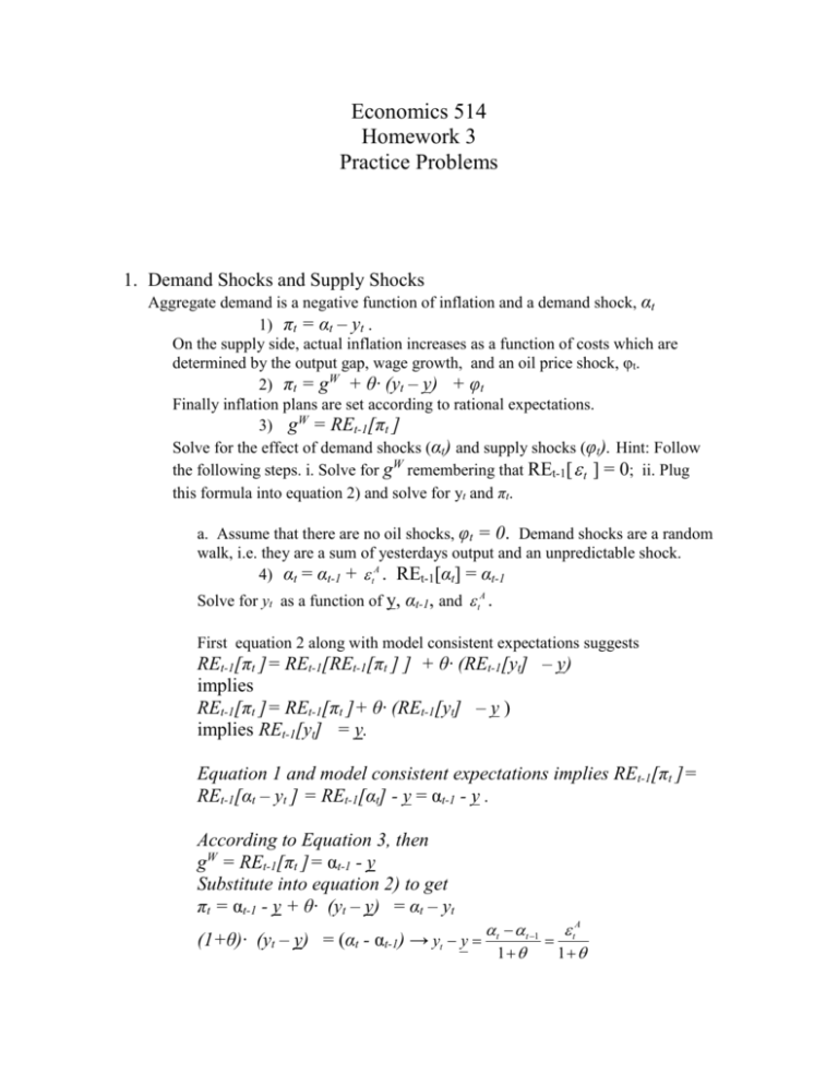
Economics 514
Homework 3
Practice Problems
1. Demand Shocks and Supply Shocks
Aggregate demand is a negative function of inflation and a demand shock, αt
1) πt = αt – yt .
On the supply side, actual inflation increases as a function of costs which are
determined by the output gap, wage growth, and an oil price shock, φt.
2) πt = gW + θ∙ (yt – y) + φt
Finally inflation plans are set according to rational expectations.
3) gW = REt-1[πt ]
Solve for the effect of demand shocks (αt) and supply shocks (φt). Hint: Follow
the following steps. i. Solve for gW remembering that REt-1[  t ] = 0; ii. Plug
this formula into equation 2) and solve for yt and πt.
a. Assume that there are no oil shocks, φt = 0. Demand shocks are a random
walk, i.e. they are a sum of yesterdays output and an unpredictable shock.
4) αt = αt-1 +  tA . REt-1[αt] = αt-1
Solve for yt as a function of y, αt-1, and  tA .
First equation 2 along with model consistent expectations suggests
REt-1[πt ]= REt-1[REt-1[πt ] ] + θ∙ (REt-1[yt] – y)
implies
REt-1[πt ]= REt-1[πt ]+ θ∙ (REt-1[yt] – y )
implies REt-1[yt] = y.
Equation 1 and model consistent expectations implies REt-1[πt ]=
REt-1[αt – yt ] = REt-1[αt] - y = αt-1 - y .
According to Equation 3, then
gW = REt-1[πt ]= αt-1 - y
Substitute into equation 2) to get
πt = αt-1 - y + θ∙ (yt – y) = αt – yt
(1+θ)∙ (yt – y) = (αt - αt-1) → yt  y 
 t   t 1  tA

1
1
b. Assume that there are no demand shocks, αt = 0. Oil shocks follow a
random walk.
5) φt = φt-1 +  tO . REt-1[φt] = φt-1
Solve for yt as a function of y, φt-1, and  tO .
First equation 2 along with model consistent expectations suggests
REt-1[πt ]= REt-1[REt-1[πt ] ] + θ∙ (REt-1[yt] – y) + REt-1[φt]
implies
REt-1[πt ]= REt-1[πt ]+ θ∙ (REt-1[yt] – y ) + φt-1
implies REt-1[yt] = y - φt-1/ θ
This means that πt = – yt so gW = REt-1[πt ] = - y + φt-1/ θ
πt = - y + φt-1/ θ + θ∙ (yt – y) + φt = – yt
(1+θ)∙ (yt – y) = φt-1/ θ + φt-1 +  tO
1
yt  y   
t 1   tO
1

1

t 1 
 tO
1
c. Do supply or demand shocks have persistent effects on output under
rational expectations?
Only unexpected demand shocks have an effect on output.
However, even last periods oil price affects the supply decision.
2. Open Economy
Construct a small model of the economy that includes A) a Planned expenditure
curve; B) a Taylor rule; and C) an expectations augmented Philips curve
A. The planned expenditure curve has two parts. The first part sets domestic
demand as a negative function of the real interest rate and an exogenous demand
shock, αt. The second part includes net exports.
yt  t  b  rt  nxt
Net exports are a function of the real exchange rate, st. The real exchange rate
adjusts so that net exports are equal to outward, capital flows that are
themselves a negative function of the gap between foreign and domestic interest
rates.
nxt  f  (st 1)  cft  g  (r f  rt )
So the expenditure curve can be written as
yt  t  b  rt  g  (r f  rt )  t  g  r f  (b  g )rt
B. The Taylor rule sets the real interest rate as an increasing function of the
inflation rate
rt  r  d  t
C.
The SRAS curve sets inflation acceleration as a function of the output gap.
 t   t 1    yt  y 
Calibrate the parameters of the model equal to r = .1, rf = .1, y= 1, b = 2 ,
d = .5, f = 2, g = 2 and θ = .5.
 t 1 = 1.2 and that at time t-1, the economy is operating at
potential output, i.e.  t 1   t 2 and yt 1  y  1 . Solve for the inflation
a. Assume that
rate, real interest rate, and real exchange rate in this economy.
Combine the expenditure curve and the Taylor rule,
yt  t  g  r f  (b  g )rt  t  g  r f  (b  g )r  d  (b  g ) t to get the
aggregate demand curve. Fill in the numbers to get
yt  t  .2  2 t
We can write
If  t 1 = 1.2 and yt 1  y  1 then 1  1.2  .2  2 t 1   t 1  0 . Then
rt 1  r  d  0  r  .1 . Then nxt 1  g  (.1  .1)  0 and
0  f  ( st 1  1)  st 1  1
b. Now, assume that at time t, an increase in fiscal spending leads to a shift
out in domestic demand and  t = 1.5. Solve for the new level of output,
real interest rate, inflation, and real exchange rate. Does the increase in
government spending cause an increase or decrease in net exports?
If
 t 1  0 then the supply curve is  t  .5  yt 1  .5 yt  .5 , so solving for
yt we write
yt  t  .2  6 t  1.5  .2  2  .5  yt 1  2.3  yt
 yt  1.15   t  .075  rt  .1375 
nxt  g  (r f  rt )  .075  st  .9625
c. Consider an alternate, extremely globalized economy with very strong
capital movements, g = 10. Now, solve for the increase in output, yt that
occurs when demand shifts from  t 1 = 1.2 to  t = 1.5. Is a globalized
economy, more or less stable in terms of output?
Combine the expenditure curve and the Taylor rule,
yt  t  g  r f  (b  g )rt  t  g  r f  (b  g )r  d  (b  g ) t to get the
aggregate demand curve. Fill in the numbers to get
yt  t  .2  6 t
We can write
If  t 1 = 1.2 and yt 1  y  1 then 1  1.2  .2  6 t 1   t 1  0 . Then
rt 1  r  d  0  r  .1 . Then nxt 1  g  (.1  .1)  0 and
0  f  ( st 1  1)  st 1  1
yt  t  .2  6 t  1.5  .2  6  .5  yt 1  4.3  3 yt
 yt  1.075   t  .0375  rt  .11875 
nxt  g  (r f  rt )  .1875  st  .90625
The openness to capital means that when government spending increases, the
increase in real interest rate draws capital sharply increasing the real
exchange rate and reducing the trade balance which offsets the rise in
government spending.
3. Rational Expectations and Persistent Shocks
Aggregate demand is given by:
6)
πt = αt – yt
where mt is (logged) money supply, αt is velocity, pt is the price level, and qt is the
output level. We will assume a fixed monetary policy. The supply curve is given by
7)
πt = gW + θ∙ (yt – y)
where gW is the growth rate of wages which is given by the expectation of the
inflation rate formed with the information available at time t-1, gW = REt-1[πt ]
and yt is the potential output level. Potential output is given by a constant, y, plus
random technology, xt.
yt  y  xt
Both supply shocks (xt) and demand shocks (αt) follow persistent movements.
 t   t 1   tD
where the innovation terms,  tD
xt   xt 1   tS
and  tS are unpredictable, so
vte   vt 1
xte   xt 1
where vte is the expectation of the time t velocity formed at time t-1 and xte is the
expectation of the time t technology formed at time t-1. Assume that expectations
are formed rationally. Normalize m = y = 0. Solve for the expectation of the output
level and the price level as a function of vt-1, xt-1, Solve for the actual output and
price level as a function of vt-1, xt-1,  tD and  tS .
Output can deviate from potential output only if actual prices to differ from expected
prices. As we cannot rationally expect the actual prices will be at some different level
from expectation, expected output must be equal to potential output. After the
normalization, the expectation of potential output is equal to
REt-1[πt ]= REt-1[REt-1[πt ] ] + θ∙ (REt-1[yt] - REt-1[xt] )
REt-1[yt] = REt-1[xt]=  xt 1
Thus, the expected inflation equals expected demand shifer minus expected output.
REt-1[πt ]=  te     t 1   xt 1 . Substituting this into the supply curve we get
 t     t 1   xt 1    yt   xt 1   tS 
The equation for the price level is  t   t  yt   t 1   tD  yt Substitute this into the
supply equation to solve for yt.
 t 1   tD  yt   t 1   xt 1    yt   xt 1   tS  
 tD   yt   xt 1     yt   xt 1   tS  

1 D
t 
1
1
 D 
 S
 t   t 1 
 t   xt 1 
t
1
1   

yt   xt 1 
 tS 
4. Baumol-Tobin Model
An econometrician estimates a version of the Baumol Tobin Model of money
demand. Her results suggest that velocity can be written as a function of the nominal
interest rate Vt  14 i . Assume the real interest rate is equal to the real output growth
rate. What is the seignorage maximizing growth rate of the money supply? What
percentage of output can possibly be collected as seignorage?
In the long run, if the real interest rate is equal to the real growth rate, the
nominal interest rate is equal to the money growth rate. Seignorage is equal to
S ( gM ) 
gM
gM M
gM Q
gM Q


4

4
Q
1 g M P 1 g M V
1 g M i
1 g M
1
S '( g M )  0  2
gM
1 g M
4
gM
1  g 
M
2

1
gM

 g M  1  S (1)  2Q
M
2 1 g
5. Okun’s Law and Time Consistency
Each % point increase in output above potential output results in θ% extra inflation.
 t  REt 1  t     yt  y 
Each % point increase in output above potential output reduces unemployment below
the natural rate by ψ%.


urt  ur NR   yt  y   t  REt 1  t   

ur  ur NR 
 t
The government is interested in low inflation and pushing unemployment toward
some target level ur*. The government sets inflation policy to minimize
2
2
a  t   b  urt  ur *
subject to  t  REt 1  t   

urt  ur NR  taking expectations as given.


a. Calculate the optimal inflation policy, πP, as a function of ur*, urNR, and
REt 1  t  .



2
2
min a  t   b  urt  ur *    REt 1  t    urt  ur NR    t 



FOC

a P
  urt  ur * 


b


 P  REt 1  t     urt  ur NR    urt  ur *  ur * ur NR 


2b  urt  ur *  
2a P   ,

 P  REt 1  t   


ur


 a  P
  ur * ur NR  

 b

 ur * 
1
REt 1  t 
a
a 2
1
1
b2
b2
b. What will equilibrium inflation and unemployment be when   REt 1  t    P
Rational expectations suggests that when inflation is set according to a predictable
policy, that policy will be incorporated into expectations. Thus, inflation will not push
output above potential output. So unemployment will equal the natural rate. Then
P 
2
NR
equilibrium inflation is


 
P
1
a
b2
2
ur
NR


ur NR  ur *
1
P
P
.
 ur * 
  
a
a 2
1
b
b2

c. If the government can choose a target unemployment rate, ur*, in order to have
zero inflation, what would it be?
Whenever the government has a bias toward unemployment below the natural rate,
inflation policy will require positive inflation. Therefore if ur* = urNR, then
equilibrium inflation is zero.