Using VLookup
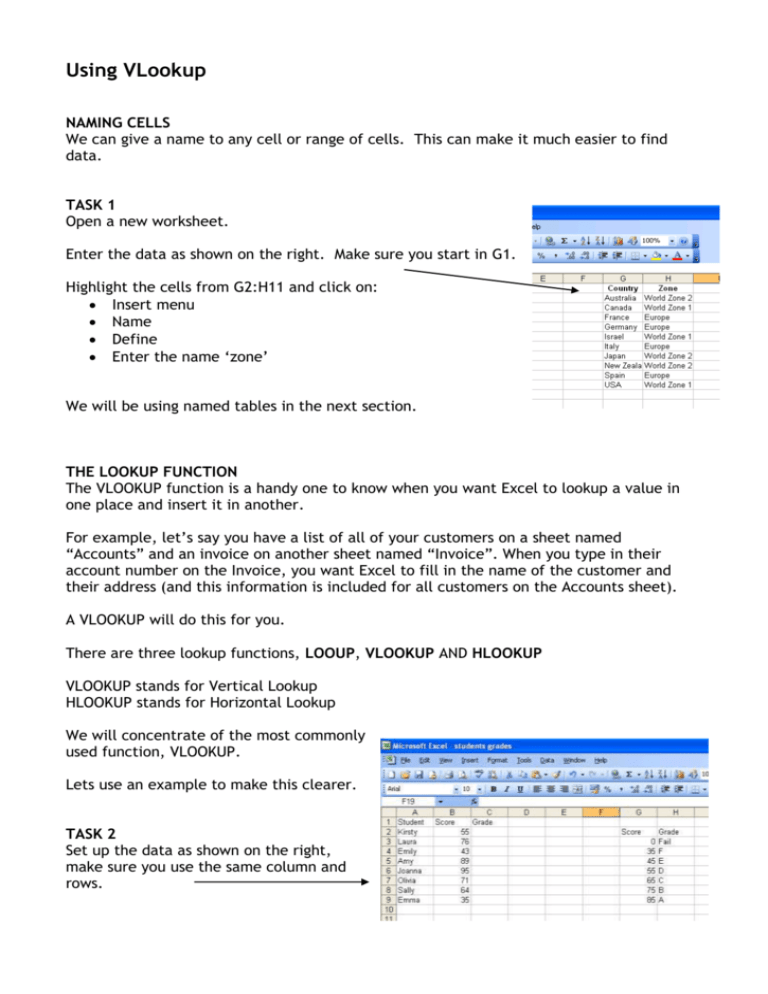
NAMING CELLS
We can give a name to any cell or range of cells. This can make it much easier to find
data.
TASK 1
Open a new worksheet.
Enter the data as shown on the right. Make sure you start in G1.
Highlight the cells from G2:H11 and click on:
 Insert menu
 Name
 Define
 Enter the name ‘zone’
We will be using named tables in the next section.
THE LOOKUP FUNCTION
The VLOOKUP function is a handy one to know when you want Excel to lookup a value in
one place and insert it in another.
For example, let’s say you have a list of all of your customers on a sheet named
“Accounts” and an invoice on another sheet named “Invoice”. When you type in their
account number on the Invoice, you want Excel to fill in the name of the customer and
their address (and this information is included for all customers on the Accounts sheet).
A VLOOKUP will do this for you.
There are three lookup functions, LOOUP, VLOOKUP AND HLOOKUP
VLOOKUP stands for Vertical Lookup
HLOOKUP stands for Horizontal Lookup
We will concentrate of the most commonly
used function, VLOOKUP.
Lets use an example to make this clearer.
TASK 2
Set up the data as shown on the right,
make sure you use the same column and
rows.
Our students have been given an exam mark. Their teacher wants an easy way to find out
which grade they should be assigned.
It is much easier to use a VLOOKUP if the table you want to look up from has been named.
Highlight cells G3:H9
Name these cells as ‘grades’
You are going to write your VLOOKUP formula in cell C2. You want to look at the mark
that Kirsty gained and find out which grade she should be given.
Click into cell C2
Click the fx icon
This screen will appear.
Click on the arrow next to category and select ‘all’ in order to get all
of the functions to appear.
In the section called ‘select a function’ scroll down until you see
VLOOKUP, click it and then click OK.
This screen will appear:
In the first section ‘Lookup_Value’ you need to tell it
what you want to look up.
Click on the blue and red button to the left hand side of
the section.
This will allow you to see your tables.
The ‘Function Argument’ box will
appear
Click into B2 and press ‘Enter’. If Enter doesn’t close the Function Argument box then
press the red cross.
B2 should now appear in the ‘Lookup_value’
In ‘Table_array’ you need to enter the name of the lookup table that you created, in this
case it is grades
The third section, ‘Col_index_num’ is asking which column you would like to return. If you
look at your grades table, it is column 2 (you will find with most lookup formulas that you
are asked to write, it is usually column 2).
Notice the last box is labeled "Range_lookup" and it is the only label that is not bold.
Whenever a label in this wizard is not bold, that means this "argument" of the function is
not required, so you can leave this blank if you choose to.
However, if you do not enter anything in this box, Excel will apply the default. If you read
the instructions at the bottom of this box, you will see that the default for this box is
"true" which will find the "closest match", whereas "false" will find an "exact match". We
are going to leave it blank this time.
Your VLOOKUP formula should look like this:
Press ‘OK’
You should find that D is returned in cell C2.
Drag the VLOOKUP formula down to cells C3:C9
You should have the following results:
Kirsty
Laura
Emily
Amy
Joanna
Olivia
Sally
Emma
55 D
76 B
43 F
89 A
95 A
71 C
64 D
35 F
Lets try another example.
TASK 3
Open a new worksheet.
Enter the data as shown on the
right. Make sure that you use
the same columns and rows.
Draw a border around your
tables – use a thicker outline and
thinner gridlines.
Centre align B:3:C:10 and F3:F7.
Use different background colours for each table.
Make the headings bold as shown.
Highlight cells F3:G7 and name the table sizes
You are going to write your VLOOKUP formula in cell C3. You will be looking at B3, and
comparing it against the table you named as ‘sizes’ and then returning the correct value in
C3.
Click on the Fx button.
Find VLOOKUP.
Lookup_Value – which cell are you looking at?
Table_array – what did you name your table?
Col_index_num – do you want column 1 or 2 to display? (remember it is usually column 2)
Have a go at the formula and see what happens.
Mr Smith should have a ‘medium’ waist.
Drag the formula down for cells C4:C10
The formula should have looked something like this:
And your results should be these:
Customer Waist size
Mr Smith
33
Mr Jameson
29
Mr Peters
34
Mr Brown
39
Mr Fletcher
46
Mr Field
52
Mr Payton
35
Mr Edmunds
30
Size
Medium
Small
Medium
Medium
Large
XL
Medium
Medium
TASK 4
Modify the Marks spreadsheet (TASK 2) so that it not only looks up the associated grade
letter, but also a suitable comment.
EXAMPLE: 80-100 Comment should be "Excellent Work!", 70 - 80 "Good Work", etc.
TASK 5 – BONUS
Using your CD-Royalty Spreadsheet, use the Royalty Rate to give one of three possible
comments: High, Medium, Low. Put this in a column that you insert between the Rate and
the Payment columns. You decide what the high, medium and low amounts should be, but
an example of each should appear in the new column.